Three dimensional (xyz) with real surface
3D Meso-NH simulations capture full spatial dynamics, including complex interactions between terrain, convection, and surface heterogeneity. They allow to study organized atmospheric structures that 1D or 2D models cannot represent. In this example you will use idealized initial condition and real surface condition.
To perform a 3D simulation with Meso-NH with idealized initial condition and real surface condition you need to prepare the physiographic data, prepare the initial condition and run the model using the PREP_PGD, PREP_IDEAL_CASE and MESONH executables respectively. In this example you will also use the DIAG program to calculate diagnostics after the simulation. These steps are described in the following sections:
Warning
This kind of simulation is parallelized and can be run with more than 1 core.
Note
You can find all the namelists presented in this section as well as the scripts here:
MNH-V6-1-0/examples/tutorials/ideal_cases/3D_real_surface/
001_prep_pgd : directory to prepare the physiographic data
002_prep_ideal_case : directory to prepare the initial condition
003_mesonh : directory to run the model
004_diag : directory to calculate diagnostics after the simulation
005_python : directory to plot the figure
The different steps must be performed in the order indicated by the directory numbers.
Prepare the physiographic data (PREP_PGD)
To create the physiographic file for a 3D Meso-NH simulation you have to use PREP_PGD program. This program reads a file called PRE_PGD1.nam defining the characteristics of the simulation.
Tip
To see all the namelists you can use in the PREP_PGD program or to obtain information about namelists, please go here.
In the PRE_PGD1.nam file, we recommend to have the following minimum informations and namelists:
The name of the NetCDF file you will create with the PREP_PGD program (without the extension) in NAM_PGDFILE namelist:
&NAM_PGDFILE CPGDFILE = "PGD" /
Note
In this example, you will create a NetCDF file
PGD.nccorresponding to surface boundary conditions files.The kind of desired projection you will use in NAM_PGD_GRID namelist:
&NAM_PGD_GRID CGRID = "CONF PROJ" /
Note
In this example, you will use conformal projection and you also need to define charastetics of this projection filling NAM_CONF_PROJ and NAM_CONF_PROJ_GRID namelists.
The characteristic of the conformal projection in NAM_CONF_PROJ namelist:
&NAM_CONF_PROJ XLAT0 = -21.125,
               XLON0 = 55.5,
               XRPK  = 0.,
               XBETA = 0. /
The characteristic of the conformal projection grid in NAM_CONF_PROJ_GRID namelist:
&NAM_CONF_PROJ_GRID XLATCEN = -21.125,
                    XLONCEN = 55.5,
                    NIMAX   = 50,
                    NJMAX   = 50,
                    XDX     = 2000.,
                    XDY     = 2000. /
Note
In this example, you will use a grid of 50x50 horizontal grid points, with a horizontal resolution of 2 km and the domain will be centered in La Reunion Island (lon=55.5, lat=-21.125).
The kind of cover database you want to use in NAM_COVER namelist:
&NAM_COVER YCOVER         = "ECOCLIMAP_v2.0",
           YCOVERFILETYPE = "DIRECT" /
Note
In this example, you will use ECOCLIMAP_v2.0 database with more than 200 covers at 1 km horizontal resolution. Other database can be found here.
The kind of orography database you want to use in NAM_ZS namelist:
&NAM_ZS YZS         = "gtopo30",
        YZSFILETYPE = "DIRECT" /
Note
In this example, you will use gtopo30 database at approximately 1 km horizontal resolution. Other database can be found here.
The kind of clay and sand database you want to use in NAM_ISBA namelist:
&NAM_ISBA YCLAY         = "CLAY_HWSD_MOY",
          YCLAYFILETYPE = "DIRECT",
          YSAND         = "SAND_HWSD_MOY",
          YSANDFILETYPE = "DIRECT" /
Note
In this example, you will use CLAY_HWSD_MOY and SAND_HWSD_MOY database at 1 km horizontal resolution. Other database can be found here.
Tip
See the full PRE_PGD1.nam file:
&NAM_PGDFILE CPGDFILE = "PGD" /

&NAM_PGD_GRID CGRID = "CONF PROJ" /

&NAM_CONF_PROJ XLAT0 = -21.125,
               XLON0 = 55.5,
               XRPK  = 0.,
               XBETA = 0. /

&NAM_CONF_PROJ_GRID XLATCEN = -21.125,
                    XLONCEN = 55.5,
                    NIMAX   = 50,
                    NJMAX   = 50,
                    XDX     = 2000.,
                    XDY     = 2000. /

&NAM_COVER YCOVER         = "ECOCLIMAP_v2.0",
           YCOVERFILETYPE = "DIRECT" /

&NAM_ZS YZS         = "gtopo30",
        YZSFILETYPE = "DIRECT" /

&NAM_ISBA YCLAY         = "CLAY_HWSD_MOY",
          YCLAYFILETYPE = "DIRECT",
          YSAND         = "SAND_HWSD_MOY",
          YSANDFILETYPE = "DIRECT" /
This file is located here :
MNH-V6-1-0/examples/tutorials/ideal_cases/3D_real_surface/001_prep_pgd/.
You can launch PREP_PGD program using run_prep_pgd.sh script (execution takes less than 2 s):
cd MNH-V6-1-0/examples/tutorials/ideal_cases/3D_real_surface/001_prep_pgd/
./run_prep_pgd.sh
At the end of the PREP_PGD execution, you need to have following files:
your_run_directory/
PRE_PGD1.nam : The file you’ve created from this example
PGD.nc : The NetCDF part of the physiographic data file
OUTPUT_LISTING0 : File containing debug informations
Tip
To verify that the program has been executed correctly, you should see the following lines at the end of the OUTPUT_LISTING0 file:
***************************
* PREP_PGD ends correctly *
***************************
Prepare the initial condition (PREP_IDEAL_CASE)
To create the initial condition for a 3D Meso-NH simulation you have to use PREP_IDEAL_CASE program. This program reads a file called PRE_IDEA1.nam defining the characteristics of the simulation.
Tip
To see all the namelists you can use in the PREP_IDEAL_CASE program or to obtain information about namelists, please go here.
In the PRE_IDEA1.nam file, we recommend to have the following minimum informations and namelists:
The name of the NetCDF files you will create with the PREP_IDEAL_CASE program (without the extension) in NAM_LUNITn namelist:
&NAM_LUNITn CINIFILE = "INI" /
Note
In this example, you will create a NetCDF file
INI.nccorresponding to initial condition file.The information about PGD file created in previous section in NAM_REAL_PGD namelist:
&NAM_REAL_PGD CPGD_FILE          = "PGD",
              LREAD_ZS           = .TRUE.,
              LREAD_GROUND_PARAM = .TRUE. /
The vertical grid discretisation in NAM_VER_GRID namelist:
&NAM_VER_GRID NKMAX   = 50,
              ZDZGRD  = 50.,
              ZDZTOP  = 700.,
              ZSTRGRD = 2500.,
              ZSTRGRD = 9.,
              ZSTRTOP = 7. /
Note
In this example, you will use 50 vertical grid points with a vertical resolution of 50 m close to the ground and a strecthing until the top of the domain with a maximum grid spacing of 700 m.
The kind of lateral boundary condition in NAM_LBCn_PRE namelist:
&NAM_LBCn_PRE CLBCX = 2*"OPEN",
              CLBCY = 2*"OPEN" /
Note
In this example, you will use open lateral boundary condition.
The surface representation in NAM_PREP_ISBA and NAM_PREP_SEAFLUX namelists:
&NAM_PREP_ISBA XTG_SURF  = 301.,
               XTG_ROOT  = 301.,
               XTG_DEEP  = 301.,
               XHUG_SURF = 0.5,
               XHUG_ROOT = 0.5,
               XHUG_DEEP = 0.5 /

&NAM_PREP_SEAFLUX XSST_UNIF = 300. /
Note
In this example, you will define some constants needed for SURFEX, XTG and XHUG correspond to ground temperature and humidity in three soil layers. XSST_UNIF correspond to uniform sea surface temperature of 300 K.
The type of initial profile and the shape of the orography you will impose in NAM_CONF_PRE :
&NAM_CONF_PRE CIDEAL = "CSTN" /
Note
In this example, you will use initialization from constant moist Brunt Vaisala frequency (
CIDEAL="CSTN").Characteristic of radiosounding has to be defined in the freeformat part of the
PRE_IDEA1.namfile (cf below).
The characteristic of the vertical profile is given in the freeformat part of the
PRE_IDEA1.namfile:CSTN 2000 01 01 0. 3 300. 100000. 0. 1000. 20000. 10. 20. 20. 0. 0. 0. 0. 0. 0. 0.007 0.01
Note
In this example you will impose an u-wind speed of 10 m/s to 20 m/s, a relative humidty of 0 % (dry simulation) and a moist brunt vaisala frequency of 0.007 and 0.01.
Tip
See the full PRE_IDEA1.nam file:
&NAM_LUNITn CINIFILE = "INI" /
&NAM_REAL_PGD CPGD_FILE = "PGD",
LREAD_ZS = .TRUE.,
LREAD_GROUND_PARAM = .TRUE. /
&NAM_VER_GRID NKMAX = 50,
ZDZGRD = 50.,
ZDZTOP = 700.,
ZSTRGRD = 2500.,
ZSTRGRD = 9.,
ZSTRTOP = 7. /
&NAM_LBCn_PRE CLBCX = 2*"OPEN",
CLBCY = 2*"OPEN" /
&NAM_PREP_ISBA XTG_SURF = 301.,
XTG_ROOT = 301.,
XTG_DEEP = 301.,
XHUG_SURF = 0.5,
XHUG_ROOT = 0.5,
XHUG_DEEP = 0.5 /
&NAM_PREP_SEAFLUX XSST_UNIF= 300. /
&NAM_CONF_PRE CIDEAL = "CSTN" /
CSTN
2000 01 01 0.
3
300.
100000.
0. 1000. 20000.
10. 20. 20.
0. 0. 0.
0. 0. 0.
0.007 0.01
This file is located here :
MNH-V6-1-0/examples/tutorials/ideal_cases/3D_real_surface/002_prep_ideal_case/.
You can launch PREP_IDEAL_CASE program using run_prep_ideal_case.sh script (execution takes less than 4 s):
cd MNH-V6-1-0/examples/tutorials/ideal_cases/3D_real_surface/002_prep_ideal_case/
./run_prep_ideal_case.sh
At the end of the PREP_IDEAL_CASE execution, you need to have following files:
your_run_directory/
PRE_IDEA1.nam : The file you’ve created from this example
INI.des : The descriptive part of the initial condition file
INI.nc : The NetCDF part of the initial condition file
PGD.nc : The NetCDF part of the physiographic data file
OUTPUT_LISTING1 : File containing debug informations
Tip
To verify that the program has been executed correctly, you should see the following lines at the end of the OUTPUT_LISTING1 file:
****************************************************
* PREP_IDEAL_CASE: PREP_IDEAL_CASE ENDS CORRECTLY. *
****************************************************
Launch the simulation (MESONH)
To launch the Meso-NH simulation you have to use MESONH program. This program reads a file called EXSEG1.nam defining the characteristics of the simulation.
Tip
To see all the namelists you can use in the MESONH program or to obtain information about namelists, please go here.
In the EXSEG1.nam file, we recommend to have the following minimum informations and namelists:
The name of the NetCDF files created by the PREP_IDEAL_CASE program in NAM_LUNITn namelist:
&NAM_LUNITn CINIFILE    = "INI",
            CINIFILEPGD = "PGD" /
The simulated length (in s), the activation of Coriolis effect, the top absorbing layer coefficient and the activation of numerical diffusion in NAM_DYN namelist :
&NAM_DYN XSEGLEN  = 600.,
         LCORIO   = .FALSE.,
         LNUMDIFU = .TRUE.,
         XALKTOP  = 0.01,
         XALZBOT  = 14000. /
The backup output writing period in NAM_BACKUP namelist:
&NAM_BACKUP XBAK_TIME(1,1) = 600.0 /
The time step, pressure solver option and the activation of the top absorbing layer in NAM_DYNn namelist:
&NAM_DYNn XTSTEP    = 10.,
          CPRESOPT  = "CRESI",
          LVE_RELAX = .TRUE.,
          XT4DIFU   = 500. /
The temporal and advection schemes in NAM_ADVn namelist:
&NAM_ADVn CTEMP_SCHEME    = "RKC4",
          CUVW_ADV_SCHEME = "CEN4TH",
          CMET_ADV_SCHEME = "PPM_01" /
The physical parametrization options in NAM_PARAMn namelist:
&NAM_PARAMn CTURB  = "TKEL",
            CRAD   = "ECMW",
            CCLOUD = "ICE3",
            CSCONV = "EDKF",
            CDCONV = "NONE" /
Note
In this example, you will use turbulence, radiative, miscrophysics and shallow convection parametrizations.
The lateral boundary condition options NAM_LBCn namelist:
&NAM_LBCn CLBCX = 2*"OPEN",
          CLBCY = 2*"OPEN" /
Note
In this example you will use open boundary condition in i and j directions.
Tip
See the full EXSEG1.nam file:
&NAM_LUNITn CINIFILE    = "INI" ,
            CINIFILEPGD = "PGD" /

&NAM_DYN XSEGLEN  = 600.,
         LCORIO   = .FALSE.,
         LNUMDIFU = .TRUE.,
         XALKTOP  = 0.01,
         XALZBOT  = 14000. /

&NAM_BACKUP XBAK_TIME(1,1) = 600. /

&NAM_DYNn XTSTEP    = 10.,
          CPRESOPT  = "CRESI",
          LVE_RELAX = .TRUE.,
          XT4DIFU   = 500. /

&NAM_ADVn CTEMP_SCHEME    = "RKC4",
          CUVW_ADV_SCHEME = "CEN4TH",
          CMET_ADV_SCHEME = "PPM_01" /

&NAM_PARAMn CTURB  = "TKEL",
            CRAD   = "ECMW",
            CCLOUD = "ICE3",
            CSCONV = "EDKF",
            CDCONV = "NONE" /

&NAM_LBCn CLBCX = 2*"OPEN",
          CLBCY = 2*"OPEN" /
This file is located here :
MNH-V6-1-0/examples/tutorials/ideal_cases/3D_real_surface/003_mesonh/.
You can launch MESONH program using run_mesonh.sh script (execution takes approximately 1 min 30 on 2 cores):
cd MNH-V6-1-0/examples/tutorials/ideal_cases/3D_real_surface/003_mesonh/
./run_mesonh.sh
At the end of the MESONH execution, you need to have following files:
your_run_directory/
INI.des : The descriptive part of the initial condition file
INI.nc : The NetCDF part of the initial condition file
PGD.nc : The NetCDF part of the physiographic data file
EXSEG1.nam : The file you’ve created from this example
EXP01.1.SEG01.000.des : The descriptive part of the simulated output file
EXP01.1.SEG01.000.nc : The NetCDF part of the simulated output file
EXP01.1.SEG01.001.des : The descriptive part of the simulated output file
EXP01.1.SEG01.001.nc : The NetCDF part of the simulated output file
OUTPUT_LISTING0 : File containing debug informations
OUTPUT_LISTING1 : File containing debug informations
Tip
The *.001.nc file contains NAM_BACKUP output. This file can be used to restart the simulation. It contains one time variables.
To verify that the program has been executed correctly, you should see the following lines at the end of the
OUTPUT_LISTING1file:|++++++++++++++++++++++++++++++++++++++++++++++++++++++++++++++++++++++++++++++++++++++++++++++++++++| | MODEL1 | CPUTIME || 137.525| 68.762| 68.702| 68.823| 100.000| | MODEL1 | ELAPSED || 137.654| 68.827| 68.827| 68.827| 100.000| |++++++++++++++++++++++++++++++++++++++++++++++++++++++++++++++++++++++++++++++++++++++++++++++++++++| |++++++++++++++++++++++++++++++++++++++++++++++++++++++++++++++++++++++++++++++++++++++++++++++++++++| |++++++++++++++++++++++++++++++++++++++++++++++++++++++++++++++++++++++++++++++++++++++++++++++++++++| |====================================================================================================| | SECOND/STEP=61 | CPUTIME || 2.255| 1.127| 1.126| 1.128| 1.639| | SECOND/STEP=61 | ELAPSED || 2.257| 1.128| 1.128| 1.128| 1.639| |----------------------------------------------------------------------------------------------------| | MICROSEC/STP/PT=125000 | CPUTIME || 18.036| 9.018| 9.010| 9.026| 100.000| | MICROSEC/STP/PT=125000 | ELAPSED || 18.053| 9.027| 9.026| 9.027| 100.000| |====================================================================================================|
Compute diagnostics after the simulation (DIAG)
To compute diagnostics after a Meso-NH simulation you have to use DIAG program. This program reads a file called DIAG1.nam defining the characteristics of the diagnostics you want.
Tip
To see all the namelists you can use in the DIAG program or to obtain information about namelists, please go here.
In the DIAG1.nam file, we recommend to have the following minimum informations and namelists:
The name of input NetCDF files and the extension of the one created by the DIAG program in NAM_DIAG_FILE namelist:
&NAM_DIAG_FILE YINIFILE(1)    = "EXP01.1.SEG01.001",
               YINIFILEPGD(1) = "PGD",
               YSUFFIX        = "diag" /
Note
In this example, you will create a file called
EXP01.1.SEG01.001diag.nc.
The type of diag you want to perform in NAM_DIAG namelist :
&NAM_DIAG LISOAL    = .TRUE.,
          XISOAL(1) = 3000.0 /
Note
In this example, you will interpole some variables at a constant altitude of 3000 m above sea level.
Tip
See the full DIAG1.nam file:
&NAM_DIAG_FILE YINIFILE(1)    = "EXP01.1.SEG01.001",
               YINIFILEPGD(1) = "PGD",
               YSUFFIX        = "diag" /

&NAM_DIAG LISOAL    = .TRUE.,
          XISOAL(1) = 3000.0 /
This file is located here :
MNH-V6-1-0/examples/tutorials/ideal_cases/3D_real_surface/004_diag/.
You can launch DIAG program using run_diag.sh script (execution takes less than 15 s):
cd MNH-V6-1-0/examples/tutorials/ideal_cases/3D_real_surface/004_diag/
./run_diag.sh
At the end of the DIAG execution, you need to have following files:
your_run_directory/
PGD.nc : The NetCDF part of the physiographic data file
DIAG1.nam : The file you’ve created from this example
EXP01.1.SEG01.001.des : The descriptive part of the simulated output file
EXP01.1.SEG01.001.nc : The NetCDF part of the simulated output file
EXP01.1.SEG01.001diag.nc : The NetCDF part of the diagnostic output file
OUTPUT_LISTING0 : File containing debug informations
OUTPUT_LISTING1 : File containing debug informations
Tip
To verify that the program has been executed correctly, you should see the following lines at the end of the OUTPUT_LISTING0 file:
***************************** **************
*            EXIT  DIAG CORRECTLY          *
**************************** ***************
Plot results
You can plot the results using run_python.sh script (execution takes less than few seconds):
cd MNH-V6-1-0/examples/tutorials/ideal_cases/3D_real_surface/005_python/
./run_python.sh
The figure created visible below shows an example of a graph that you can plot from the 3D simulation you just performed. It shows the zonal wind speed at 3000 m a.s.l. perturbed by the orography. Contours correspond to isoaltiudes levels and are used to show Reunion Island.
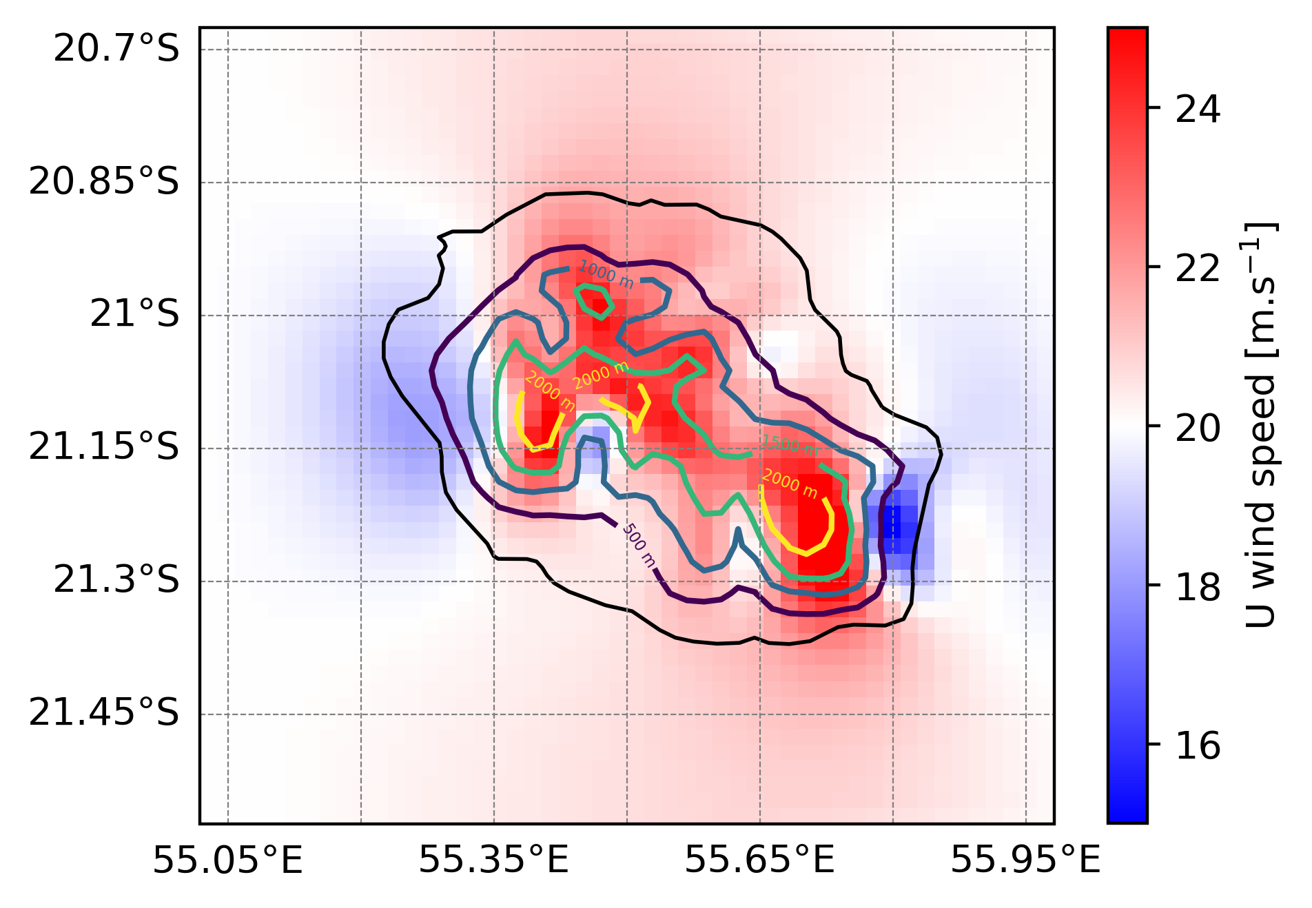
Example of 3D simulation output. U wind speed at 3000 m a.s.l.
Tip
See the python script used to plot this figure:
#!/usr/bin/python
# -*- coding: utf-8 -*-

# ~~~~~~~~~~~~~~~~~~~~~~~~~~~~~~~~~~~~~~~~~~~~~~~~~~~~~~~~~
import numpy as np
import netCDF4
import matplotlib.pyplot as plt
import cartopy.crs as ccrs
# ~~~~~~~~~~~~~~~~~~~~~~~~~~~~~~~~~~~~~~~~~~~~~~~~~~~~~~~~~

# #########################################################
# ###           To be defined by user                   ###
# #########################################################

cfg_file_name = 'EXP01.1.SEG01.001diag.nc'

# #########################################################

# ------------------------------------------------------
#   Read netcdf file and variables
# ------------------------------------------------------

file_MNH     = netCDF4.Dataset(cfg_file_name)

lon_MNH     = file_MNH['LON'][1:-1,1:-1]
lat_MNH     = file_MNH['LAT'][1:-1,1:-1]

zs_MNH       = file_MNH['ZS'][1:-1,1:-1]
uwnd_MNH     = file_MNH['ALT_U'][0,0,1:-1,1:-1]

# ------------------------------------------------------
#   Quick plot
# ------------------------------------------------------

fig = plt.figure(figsize=(5, 5))
ax  = plt.axes(projection=ccrs.PlateCarree())

pmsh = ax.pcolormesh(lon_MNH[:,:], lat_MNH[:,:], uwnd_MNH[:,:], vmin=15.0, vmax=25.0, shading="auto", cmap="bwr")
ct   = ax.contour(lon_MNH[:,:], lat_MNH[:,:], zs_MNH[:,:], levels=[500.0, 1000.0, 1500.0, 2000.0])

# ------------------------------------------------------
#   Some adjustments to the plot
# ------------------------------------------------------

gl = ax.gridlines(draw_labels=True, linewidth=0.4, color='gray', linestyle='--')
gl.top_labels = False
gl.right_labels = False

ax.coastlines()

cbar=plt.colorbar(pmsh,shrink=0.75)
cbar.set_label(r"U wind speed [m.s$^{-1}$]")

plt.clabel(ct, inline=True, fmt='%d m', fontsize=4)

plt.savefig('3D_real_surface.png', bbox_inches='tight', dpi=400)
This file is located here :
MNH-V6-1-0/examples/tutorials/ideal_cases/3D_real_surface/005_python/.
Other examples
You can find other 3D ideal simulation with real surface examples in Namelist catalogue section.