One dimensional (single column z) with ideal surface
Some of the most important advantages to use one dimensional (or single column, 1D) atmospheric simulations are :
Simplicity : simpler and require fewer computing resources than 2D or 3D models.
Study vertical processes and surface-atmosphere interactions : focus on vertical processes in the atmosphere, such as convection, cloud formation, and heat and moisture exchange without the complexity of horizontal advection.
Parameterisation development and testing : used to develop and test new physical parameterisations (e.g. for clouds, precipitation or radiation) before they are integrated into 2D or 3D models.
To perform a 1D simulation with Meso-NH you need to prepare the initial condition and run the model using the PREP_IDEAL_CASE and MESONH executables respectively. These two steps are described in the following sections:
Warning
This kind of simulation is not parallelized and can only be run on 1 core.
Note
You can find all the namelists presented in this section as well as the scripts here:
MNH-V6-1-0/examples/tutorials/ideal_cases/1D/
001_prep_ideal_case : directory to prepare the initial condition
002_mesonh : directory to run the model
003_python : directory to plot the figure
The different steps must be performed in the order indicated by the directory numbers.
Prepare the initial condition (PREP_IDEAL_CASE)
To create the initial condition for a vertical 1D Meso-NH simulation you have to use PREP_IDEAL_CASE program. This program reads a file called PRE_IDEA1.nam defining the characteristics of the simulation.
Tip
To see all the namelists you can use in the PREP_IDEAL_CASE program or to obtain information about namelists, please go here.
In the PRE_IDEA1.nam file, we recommend to have the following minimum informations and namelists:
The name of the NetCDF files you will create with the PREP_IDEAL_CASE program (without the extension) in NAM_LUNITn namelist:
&NAM_LUNITn CINIFILE    = "INI",
            CINIFILEPGD = "PGD" /
Note
In this example, you will create the two NetCDF files
INI.ncandPGD.nccorresponding respectively to initial and surface boundary conditions files.The number of points along x (i) and y (j) direction (it has to be 1 in 1D configuration) in NAM_DIMn_PRE namelist:
&NAM_DIMn_PRE NIMAX = 1,
              NJMAX = 1 /
The horizontal resolution along i and j direction in NAM_GRIDH_PRE namelist:
&NAM_GRIDH_PRE XDELTAX = 1000.,
               XDELTAY = 1000. /
Note
It is better to set XDELTAX and XDELTAY to a value that is consistent with the relevant resolution of the parameterization you are testing (at least 1000.0 (m), or even 50 000 (m) if climate applications are targeted).
The vertical grid discretisation in NAM_VER_GRID namelist:
&NAM_VER_GRID NKMAX  = 100,
              ZDZGRD = 40.,
              ZDZTOP = 40. /
Note
In this example, you will use 100 vertical grid points with a vertical resolution of 40 m everywhere.
The surface representation in NAM_GRn_PRE, NAM_PGD_SCHEMES and NAM_COVER namelists:
&NAM_GRn_PRE CSURF        = "EXTE" /
&NAM_COVER XUNIF_COVER(1) =  1.0   /
&NAM_PGD_SCHEMES CSEA     = "FLUX" /
Note
In this example, you will use SURFEX (CSURF = “EXTE”), a cover containing 100 % sea points (XUNIF_COVER(1) = 1.0) and a prescribed ideal flux surface condition (CSEA = “FLUX”).
The values of surface fluxes are given in the simulation namelist (see simulation section).
The type of initial profile you will impose in NAM_CONF_PRE:
&NAM_CONF_PRE CIDEAL = "RSOU" /
The characteristic of the vertical profile is given in the freeformat part of the
PRE_IDEA1.namfile:RSOU 2025 6 11 0. "ZUVTHVHU" 0. 100000. 305. 0. 2 0 0 0 4000 0 0 4 20.00 300.00 0.00 1000.00 300.00 0.00 4000.00 317.90 0.00
Note
In this example you will impose an horizontal wind speed of 0 m/s, a relative humidty of 0 % (dry simulation) and a constant potential temperature of 300 K from 0 m to 1000 m and then a regular increase of the potential temperature up to the top of the domain (4000 m).
Tip
See the full PRE_IDEA1.nam file:
&NAM_LUNITn CINIFILE    = "INI",
            CINIFILEPGD = "PGD" /

&NAM_DIMn_PRE NIMAX = 1,
              NJMAX = 1 /

&NAM_GRIDH_PRE XDELTAX = 1000.,
               XDELTAY = 1000. /

&NAM_VER_GRID NKMAX  = 100,
              ZDZGRD = 40.,
              ZDZTOP = 40. /

&NAM_GRn_PRE CSURF        = "EXTE" /
&NAM_COVER XUNIF_COVER(1) =  1.0   /
&NAM_PGD_SCHEMES CSEA     = "FLUX" /

&NAM_CONF_PRE CIDEAL = "RSOU" /

RSOU
2025 6 11 0.
"ZUVTHVHU"
0.
100000.
300.
0.

2
0        0      0
4000     0      0

4
  20.0     300.0  0.0
1000.0     300.0  0.0
4000.0     317.9  0.0
This file is located here :
MNH-V6-1-0/examples/tutorials/ideal_cases/1D/001_prep_ideal_case/
You can launch PREP_IDEAL_CASE program using run_prep_ideal_case.sh script (execution takes less than 2 s):
cd MNH-V6-1-0/examples/tutorials/ideal_cases/1D/001_prep_ideal_case/
./run_prep_ideal_case.sh
At the end of the PREP_IDEAL_CASE execution, you need to have following files:
MNH-V6-1-0/examples/tutorials/1D/001_prep_ideal_case/
PRE_IDEA1.nam : The namelist file from this example
INI.des : The descriptive part of the initial condition file
INI.nc : The NetCDF part of the initial condition file
PGD.nc : The NetCDF part of the physiographic data file
OUTPUT_LISTING1 : File containing debug informations
Tip
To verify that the program has been executed correctly, you should see the following lines at the end of the OUTPUT_LISTING1 file:
****************************************************
* PREP_IDEAL_CASE: PREP_IDEAL_CASE ENDS CORRECTLY. *
****************************************************
Launch the simulation (MESONH)
To launch the Meso-NH simulation you have to use MESONH program. This program reads a file called EXSEG1.nam defining the characteristics of the simulation.
Tip
To see all the namelists you can use in the MESONH program or to obtain information about namelists, please go here.
In the EXSEG1.nam file, we recommend to have the following minimum informations and namelists:
The name of the NetCDF files created by the PREP_IDEAL_CASE program in NAM_LUNITn namelist:
&NAM_LUNITn CINIFILE    = "INI",
            CINIFILEPGD = "PGD" /
The simulated length (in s) and the activation of Coriolis effect in NAM_DYN namelist :
&NAM_DYN XSEGLEN = 25200.0,
         LCORIO  = .FALSE. /
The backup output writing period in NAM_BACKUP namelist:
&NAM_BACKUP XBAK_TIME(1,1) = 25200.0 /
The time step and pressure solver option in NAM_DYNn namelist:
&NAM_DYNn XTSTEP   = 10.0,
          CPRESOPT = "ZRESI" /
The temporal and advection schemes in NAM_ADVn namelist:
&NAM_ADVn CTEMP_SCHEME    = "RKC4",
          CUVW_ADV_SCHEME = "CEN4TH",
          CMET_ADV_SCHEME = "PPM_01" /
The physical parametrization options in NAM_PARAMn namelist:
&NAM_PARAMn CTURB  = "TKEL",
            CRAD   = "NONE",
            CCLOUD = "NONE",
            CSCONV = "EDKF",
            CDCONV = "NONE" /
The turbulence scheme option in NAM_TURBn namelist:
&NAM_TURBn CTURBDIM="1DIM",
           CTURBLEN="RM17" /
Note
In this example you will use 1D version of the turbulence scheme and the mixing lentgh of Rodier et al. [2017].
The turbulence diagnostics in NAM_LES:
&NAM_LES LLES_MEAN = .TRUE. /
Note
Only the mean variables are stored in this example.
The shallow convection options in NAM_PARAM_MFSHALLn:
&NAM_PARAM_MFSHALLn CMF_UPDRAFT = "EDKF",
                    LMIXUV      = .TRUE.,
                    LMF_FLX     = .TRUE. /
Note
You will chose to use EDKF parametrization (
CMF_UPDRAFT = "EDKF"), to activate wind mixing from thermal structures (LMIXUV = .TRUE.) and to store the mass fluxes (LMF_FLX = .TRUE.).The heat fluxes imposed at the surface boundary condition in NAM_IDEAL_FLUX:
&NAM_IDEAL_FLUX NFORCF    = 2,
                XTIMEF(1) = 0.,
                XTIMEF(2) = 25200.,
                XSFTH(1)  = 200.0,
                XSFTH(2)  = 200.0 /
Note
In this example, you will force your simulation with surface constant heat flux of 200 W/m2 throughout the simulation.
Tip
See the full EXSEG1.nam file:
&NAM_LUNITn CINIFILE    = "INI" ,
            CINIFILEPGD = "PGD" /

&NAM_DYN XSEGLEN = 25200.0,
         LCORIO  = .FALSE. /

&NAM_BACKUP XBAK_TIME(1,1) = 25200.0 /

&NAM_DYNn XTSTEP   = 10.0,
          CPRESOPT = "ZRESI" /

&NAM_ADVn CTEMP_SCHEME    = "RKC4",
          CUVW_ADV_SCHEME = "CEN4TH",
          CMET_ADV_SCHEME = "PPM_01" /

&NAM_PARAMn CTURB  = "TKEL",
            CRAD   = "NONE",
            CCLOUD = "NONE",
            CSCONV = "EDKF",
            CDCONV = "NONE" /

&NAM_TURBn CTURBDIM="1DIM",
           CTURBLEN="RM17" /

&NAM_LES LLES_MEAN = .TRUE. /

&NAM_PARAM_MFSHALLn CMF_UPDRAFT = "EDKF",
                    LMIXUV      = .TRUE.,
                    LMF_FLX     = .TRUE. /

&NAM_IDEAL_FLUX NFORCF    = 2,
                XTIMEF(1) = 0.,
                XTIMEF(2) = 25200.,
                XSFTH(1)  = 200.0,
                XSFTH(2)  = 200.0 /
This file is located here :
MNH-V6-1-0/examples/tutorials/ideal_cases/1D/002_mesonh/
You can launch MESONH program using run_mesonh.sh script (execution takes less than 15 s):
cd MNH-V6-1-0/examples/tutorials/ideal_cases/1D/002_mesonh/
./run_mesonh.sh
At the end of the MESONH execution, you need to have following files:
your_run_directory/
INI.des : The descriptive part of the initial condition file
INI.nc : The NetCDF part of the initial condition file
PGD.nc : The NetCDF part of the physiographic data file
EXSEG1.nam : The file you’ve created from this example
EXP01.1.SEG01.000.des : The descriptive part of the simulated output file
EXP01.1.SEG01.000.nc : The NetCDF part of the simulated output file
EXP01.1.SEG01.001.des : The descriptive part of the simulated output file
EXP01.1.SEG01.001.nc : The NetCDF part of the simulated output file
OUTPUT_LISTING0 : File containing debug informations
OUTPUT_LISTING1 : File containing debug informations
Tip
The *.001.nc file contains NAM_BACKUP output. This file can be used to restart the simulation. It contains one time variables.
To verify that the program has been executed correctly, you should see the following lines at the end of the
OUTPUT_LISTING1file:|----------------------------------------------------------------------------------------------------| | CPUTIME/ELAPSED || SUM(PROC) |MEAN(PROC)| MIN(PROC | MAX(PROC)| PERCENT %| |----------------------------------------------------------------------------------------------------| |++++++++++++++++++++++++++++++++++++++++++++++++++++++++++++++++++++++++++++++++++++++++++++++++++++| |++++++++++++++++++++++++++++++++++++++++++++++++++++++++++++++++++++++++++++++++++++++++++++++++++++| |++++++++++++++++++++++++++++++++++++++++++++++++++++++++++++++++++++++++++++++++++++++++++++++++++++| | MODEL1 | CPUTIME || 12.142| 12.142| 12.142| 12.142| 100.000| | MODEL1 | ELAPSED || 12.159| 12.159| 12.159| 12.159| 100.000| |++++++++++++++++++++++++++++++++++++++++++++++++++++++++++++++++++++++++++++++++++++++++++++++++++++| |++++++++++++++++++++++++++++++++++++++++++++++++++++++++++++++++++++++++++++++++++++++++++++++++++++| |++++++++++++++++++++++++++++++++++++++++++++++++++++++++++++++++++++++++++++++++++++++++++++++++++++| |====================================================================================================| | SECOND/STEP=2521 | CPUTIME || 0.005| 0.005| 0.005| 0.005| 0.040| | SECOND/STEP=2521 | ELAPSED || 0.005| 0.005| 0.005| 0.005| 0.040| |----------------------------------------------------------------------------------------------------| | MICROSEC/STP/PT=100 | CPUTIME || 48.163| 48.163| 48.163| 48.163| 100.000| | MICROSEC/STP/PT=100 | ELAPSED || 48.230| 48.230| 48.230| 48.230| 100.000| |====================================================================================================|
Plot results
You can plot the results using run_python.sh script (execution takes less than few seconds):
cd MNH-V6-1-0/examples/tutorials/ideal_cases/1D/003_python/
./run_python.sh
The figure created visible below shows an example of a graph that you can plot from the 1D simulation you just performed. It shows the temporal evolution of the atmospheric boundary layer through the vertical potential temperature profile.
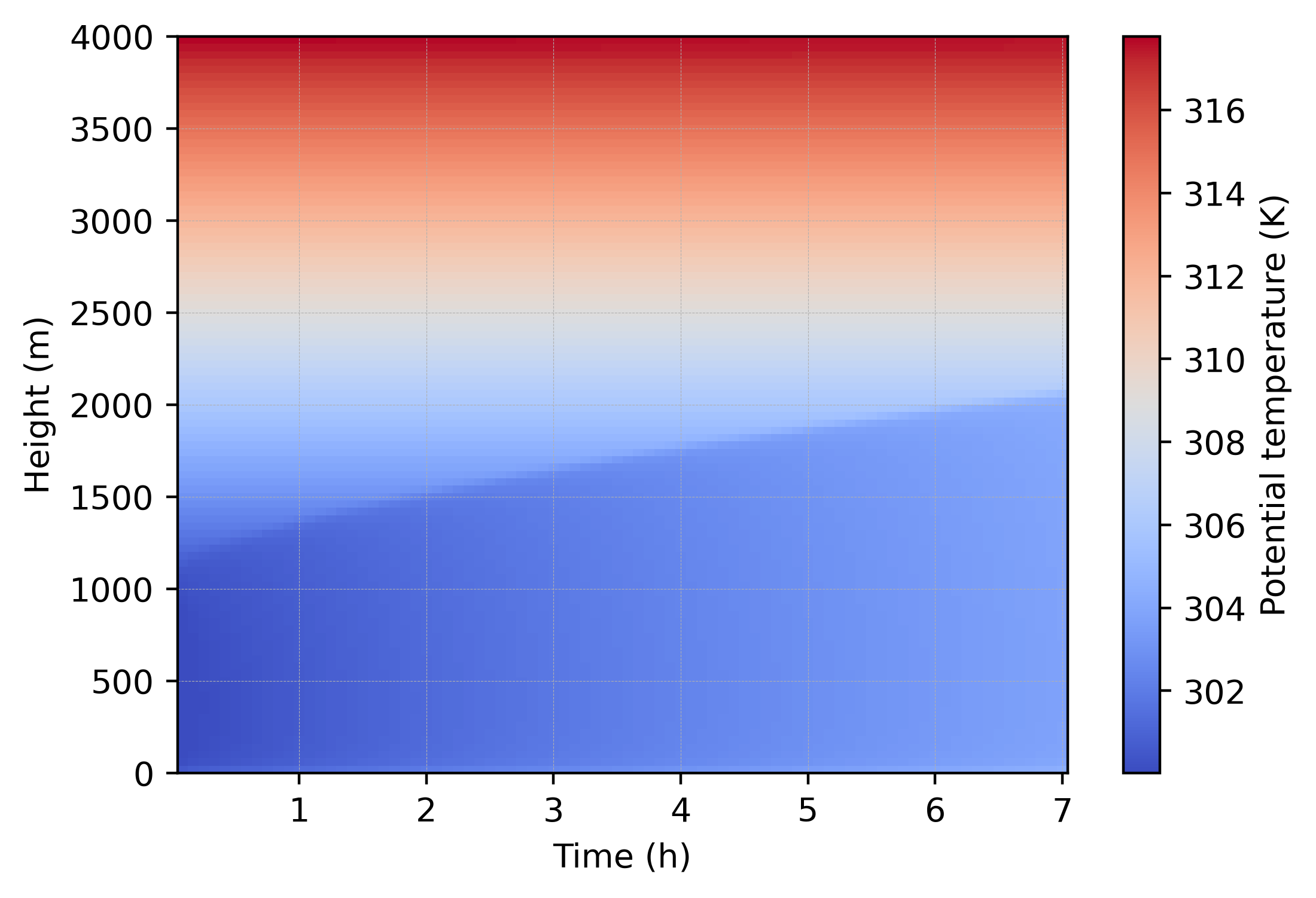
Example of 1D simulation output. Evolution of the vertical profile of potential temperature.
Tip
See the python script used to plot this figure:
#!/usr/bin/python
# -*- coding: utf-8 -*-

# ~~~~~~~~~~~~~~~~~~~~~~~~~~~~~~~~~~~~~~~~~~~~~~~~~~~~~~~~~
import numpy as np
import netCDF4
import matplotlib.pyplot as plt
# ~~~~~~~~~~~~~~~~~~~~~~~~~~~~~~~~~~~~~~~~~~~~~~~~~~~~~~~~~

# #########################################################
# ###           To be defined by user                   ###
# #########################################################

cfg_file_name = 'EXP01.1.SEG01.000.nc'

# #########################################################

# ------------------------------------------------------
#   Read netcdf file and variables
# ------------------------------------------------------

file_MNH       = netCDF4.Dataset(cfg_file_name)
time_MNH       = file_MNH['time_les'][:]/3600.0
level_MNH      = file_MNH['level_les']
mean_theta_MNH = file_MNH['LES_budgets']['Mean']['Cartesian']['Not_time_averaged']['Not_normalized']['cart']['MEAN_TH']

# ------------------------------------------------------
#   Quick plot
# ------------------------------------------------------

plt.pcolormesh(time_MNH[:], level_MNH, np.transpose(mean_theta_MNH), shading="auto", cmap="coolwarm")

# ------------------------------------------------------
#   Some adjustments to the plot
# ------------------------------------------------------

plt.grid(True, linestyle='--', linewidth=0.2)

cbar=plt.colorbar()
cbar.set_label("Potential temperature (K)")

plt.xlabel("Time (h)")
plt.ylabel("Height (m)")

plt.savefig('1D.png', bbox_inches='tight', dpi=400)
This file is located here :
MNH-V6-1-0/examples/tutorials/ideal_cases/1D/003_python/
Other examples
You can find other 1D simulation examples in Namelist catalogue section.