Two dimensional (cross-section xz or yz) with ideal surface
2D simulation is a powerful compromise between 1D and 3D simulations : it retains both horizontal and vertical dimensions, allowing a large number of atmospheric phenomena to be represented without the significant cost of a 3D simulation. 2D configurations are able to study free convection, thermals, gravity waves, 2D turbulence, …
To perform a 2D simulation with Meso-NH you need to prepare the initial condition and run the model using the PREP_IDEAL_CASE and MESONH executables respectively. These two steps are described in the following sections:
Warning
This kind of simulation is not parallelized and can only be run on 1 core.
Note
You can find all the namelists presented in this section as well as the scripts here:
MNH-V6-1-0/examples/tutorials/ideal_cases/2D/
001_prep_ideal_case : directory to prepare the initial condition
002_mesonh : directory to run the model
003_python : directory to plot the figure
The different steps must be performed in the order indicated by the directory numbers.
Prepare the initial condition (PREP_IDEAL_CASE)
To create the initial condition for a 2D Meso-NH simulation you have to use PREP_IDEAL_CASE program. This program reads a file called PRE_IDEA1.nam defining the characteristics of the simulation.
Tip
To see all the namelists you can use in the PREP_IDEAL_CASE program or to obtain information about namelists, please go here.
In the PRE_IDEA1.nam file, we recommend to have the following minimum informations and namelists:
The name of the NetCDF files you will create with the PREP_IDEAL_CASE program (without the extension) in NAM_LUNITn namelist:
&NAM_LUNITn CINIFILE    = "INI",
            CINIFILEPGD = "PGD" /
Note
In this example, you will create the two NetCDF files
INI.ncandPGD.nccorresponding respectively to initial and surface boundary conditions files.The number of points along x (i) and y (j) direction (it has to be 1 for one direction for 2D configuration) in NAM_DIMn_PRE namelist:
&NAM_DIMn_PRE NIMAX = 200,
              NJMAX = 1 /
Note
In this example, you will have a x-z domain.
The type of initial profile and the shape of the orography you will impose in NAM_CONF_PRE :
&NAM_CONF_PRE CIDEAL = "RSOU",
              CZS    = "BELL" /
Note
In this example, you will use initialization from radiosounding (
CIDEAL="RSOU") and bell-shape hill orography (CZS="BELL").Characteristic of radiosounding has to be defined in the freeformat part of the
PRE_IDEA1.namfile (cf below).Characteristic of the bell-shape hill orography has to be defined in NAM_GRIDH_PRE namelist.
The horizontal resolution along i and j direction and the orography charateristic in NAM_GRIDH_PRE namelist:
&NAM_GRIDH_PRE XDELTAX = 2000.,
               XDELTAY = 2000.,
               XHMAX   = 100.,
               XAX     = 8000.,
               NIZS    = 100 /
Note
It is better to set XDELTAX and XDELTAY to a value that is consistent with the relevant resolution of the your case study. XHMAX, XAX and NIZS correspond to characteristic of the bell-shape hill you’ve chose in NAM_CONF_PRE namelist.
The vertical grid discretisation in NAM_VER_GRID namelist:
&NAM_VER_GRID NKMAX  = 40,
              ZDZGRD = 750.,
              ZDZTOP = 750. /
Note
In this example, you will use 40 vertical grid points with a vertical resolution of 750 m everywhere.
The kind of lateral boundary condition in NAM_LBCn_PRE namelist:
&NAM_LBCn_PRE CLBCX(1) = "CYCL",
              CLBCX(2) = "CYCL" /
Note
In this example, you will use cyclic lateral boundary condition in PREP_IDEAL_CASE to impose cyclic orography.
The surface representation in NAM_GRn_PRE and NAM_COVER namelists:
&NAM_GRn_PRE CSURF        = "EXTE" /
&NAM_COVER XUNIF_COVER(4) =  1.0   /
Note
In this example, you will use SURFEX (
CSURF = "EXTE") and a cover containing 100 % nature points (XUNIF_COVER(4) = 1.0).The characteristic of the vertical profile is given in the freeformat part of the
PRE_IDEA1.namfile:RSOU 2025 6 11 0. "ZUVTHVHU" 0. 100000. 288. 0. 2 0 10 0 30000 10 0 2 50.0 288.15 0.0 29900.0 390.68 0.0
Note
In this example you will impose an u-wind speed of 10 m/s, a relative humidty of 0 % (dry simulation) and a regular increase of the potential temperature from 288 K at 0 m to 390.68 K at 29900 m.
Tip
See the full PRE_IDEA1.nam file:
&NAM_LUNITn CINIFILE = "INI",
CINIFILEPGD = "PGD" /
&NAM_DIMn_PRE NIMAX = 200,
NJMAX = 1 /
&NAM_CONF_PRE CIDEAL = "RSOU",
CZS = "BELL" /
&NAM_GRIDH_PRE XDELTAX = 2000.,
XDELTAY = 2000.,
XHMAX = 100.,
XAX = 8000.,
NIZS = 100 /
&NAM_VER_GRID NKMAX = 40,
ZDZGRD = 750.,
ZDZTOP = 750. /
&NAM_LBCn_PRE CLBCX(1) = "CYCL",
CLBCX(2) = "CYCL" /
&NAM_GRn_PRE CSURF = "EXTE" /
&NAM_COVER XUNIF_COVER(4) = 1.0 /
RSOU
2025 6 11 0.
"ZUVTHVHU"
0.
100000.
288.
0.

2
0        10      0
30000    10      0

2
   50.0    288.15  0.0
29900.0    390.68  0.0
This file is located here :
MNH-V6-1-0/examples/tutorials/ideal_cases/2D/001_prep_ideal_case/
You can launch PREP_IDEAL_CASE program using run_prep_ideal_case.sh script (execution takes approximately 2 s):
cd MNH-V6-1-0/examples/tutorials/2D/001_prep_ideal_case/
./run_prep_ideal_case.sh
At the end of the PREP_IDEAL_CASE execution, you need to have following files:
MNH-V6-1-0/examples/tutorials/ideal_cases/2D/001_prep_ideal_case/
PRE_IDEA1.nam : The file you’ve created from this example
INI.des : The descriptive part of the initial condition file
INI.nc : The NetCDF part of the initial condition file
PGD.nc : The NetCDF part of the physiographic data file
OUTPUT_LISTING1 : File containing debug informations
Tip
To verify that the program has been executed correctly, you should see the following lines at the end of the OUTPUT_LISTING1 file:
****************************************************
* PREP_IDEAL_CASE: PREP_IDEAL_CASE ENDS CORRECTLY. *
****************************************************
Launch the simulation (MESONH)
To launch the Meso-NH simulation you have to use MESONH program. This program reads a file called EXSEG1.nam defining the characteristics of the simulation.
Tip
To see all the namelists you can use in the MESONH program or to obtain information about namelists, please go here.
In the EXSEG1.nam file, we recommend to have the following minimum informations and namelists:
The name of the NetCDF files created by the PREP_IDEAL_CASE program in NAM_LUNITn namelist:
&NAM_LUNITn CINIFILE    = "INI",
            CINIFILEPGD = "PGD" /
The simulated length (in s), the activation of Coriolis effect and the top absorbing layer coefficient in NAM_DYN namelist :
&NAM_DYN XSEGLEN = 36000.,
         LCORIO  = .FALSE.,
         XALKTOP = 0.005,
         XALZBOT = 20000. /
Note
To activate the top absorbing layer you have to put
LVE_RELAX = .TRUE.in NAM_DYNn namelist.The backup output writing period in NAM_BACKUP namelist:
&NAM_BACKUP XBAK_TIME(1,1) = 3600.,
            XBAK_TIME(1,2) = 12000.,
            XBAK_TIME(1,3) = 36000. /
The time step, pressure solver option and the activation of the top absorbing layer in NAM_DYNn namelist:
&NAM_DYNn XTSTEP    = 20.,
          CPRESOPT  = "CRESI",
          LVE_RELAX = .TRUE. /
The temporal and advection schemes in NAM_ADVn namelist:
&NAM_ADVn CTEMP_SCHEME    = "RKC4",
          CUVW_ADV_SCHEME = "CEN4TH",
          CMET_ADV_SCHEME = "PPM_01" /
The physical parametrization options in NAM_PARAMn namelist:
&NAM_PARAMn CTURB  = "NONE",
            CRAD   = "NONE",
            CCLOUD = "NONE",
            CSCONV = "NONE",
            CDCONV = "NONE" /
Note
In this example, no physical parameters are activated.
The lateral boundary condition options NAM_LBCn namelist:
&NAM_LBCn CLBCX = 2*"OPEN" /
Note
In this example you will use open boundary condition in i direction, by default it’s cyclic along j direction.
Tip
See the full EXSEG1.nam file:
&NAM_LUNITn CINIFILE    = "INI" ,
            CINIFILEPGD = "PGD" /

&NAM_DYN XSEGLEN = 36000.,
         LCORIO  = .FALSE.,
         XALKTOP = 0.005,
         XALZBOT = 20000. /

&NAM_BACKUP XBAK_TIME(1,1) = 3600.,
            XBAK_TIME(1,2) = 12000.,
            XBAK_TIME(1,3) = 36000. /

&NAM_DYNn XTSTEP    = 20.,
          CPRESOPT  = "CRESI",
          LVE_RELAX = .TRUE. /

&NAM_ADVn CTEMP_SCHEME    = "RKC4",
          CUVW_ADV_SCHEME = "CEN4TH",
          CMET_ADV_SCHEME = "PPM_01" /

&NAM_PARAMn CTURB  = "NONE",
            CRAD   = "NONE",
            CCLOUD = "NONE",
            CSCONV = "NONE",
            CDCONV = "NONE" /

&NAM_LBCn CLBCX = 2*"OPEN" /
This file is located here :
MNH-V6-1-0/examples/tutorials/ideal_cases/2D/002_mesonh/
Once you have put these namelist in the EXSEG1.nam file, you can launch MESONH program in the same directory as the EXSEG1.nam, INI.des, INI.nc and PGD.nc files (execution takes approximately 1 min 30):
cd MNH-V6-1-0/examples/tutorials/ideal_cases/2D/002_mesonh/
./run_mesonh.sh
At the end of the MESONH execution, you need to have following files:
your_run_directory/
INI.des : The descriptive part of the initial condition file
INI.nc : The NetCDF part of the initial condition file
PGD.nc : The NetCDF part of the physiographic data file
EXSEG1.nam : The file you’ve created from this example
EXP01.1.SEG01.000.des : The descriptive part of the simulated output file
EXP01.1.SEG01.000.nc : The NetCDF part of the simulated output file
EXP01.1.SEG01.001.des : The descriptive part of the simulated output file
EXP01.1.SEG01.001.nc : The NetCDF part of the simulated output file
OUTPUT_LISTING0 : File containing debug informations
OUTPUT_LISTING1 : File containing debug informations
Tip
The *.001.nc file contains NAM_BACKUP output. This file can be used to restart the simulation. It contains one time variables.
To verify that the program has been executed correctly, you should see the following lines at the end of the
OUTPUT_LISTING1file:|----------------------------------------------------------------------------------------------------| | CPUTIME/ELAPSED || SUM(PROC) |MEAN(PROC)| MIN(PROC | MAX(PROC)| PERCENT %| |----------------------------------------------------------------------------------------------------| |++++++++++++++++++++++++++++++++++++++++++++++++++++++++++++++++++++++++++++++++++++++++++++++++++++| |++++++++++++++++++++++++++++++++++++++++++++++++++++++++++++++++++++++++++++++++++++++++++++++++++++| |++++++++++++++++++++++++++++++++++++++++++++++++++++++++++++++++++++++++++++++++++++++++++++++++++++| | MODEL1 | CPUTIME || 93.270| 93.270| 93.270| 93.270| 100.000| | MODEL1 | ELAPSED || 93.407| 93.407| 93.407| 93.407| 100.000| |++++++++++++++++++++++++++++++++++++++++++++++++++++++++++++++++++++++++++++++++++++++++++++++++++++| |++++++++++++++++++++++++++++++++++++++++++++++++++++++++++++++++++++++++++++++++++++++++++++++++++++| |++++++++++++++++++++++++++++++++++++++++++++++++++++++++++++++++++++++++++++++++++++++++++++++++++++| |====================================================================================================| | SECOND/STEP=1801 | CPUTIME || 0.052| 0.052| 0.052| 0.052| 0.056| | SECOND/STEP=1801 | ELAPSED || 0.052| 0.052| 0.052| 0.052| 0.056| |----------------------------------------------------------------------------------------------------| | MICROSEC/STP/PT=8000 | CPUTIME || 6.474| 6.474| 6.474| 6.474| 100.000| | MICROSEC/STP/PT=8000 | ELAPSED || 6.483| 6.483| 6.483| 6.483| 100.000| |====================================================================================================|
Plot results
You can plot the results using run_python.sh script (execution takes less than few seconds):
cd MNH-V6-1-0/examples/tutorials/ideal_cases/2D/003_python/
./run_python.sh
The figure created visible below shows an example of a graph that you can plot from the 2D simulation you just performed. It shows the orographic wave generated by the 100 m bell shape hill through vertical velocity wind speed along x-z domain.
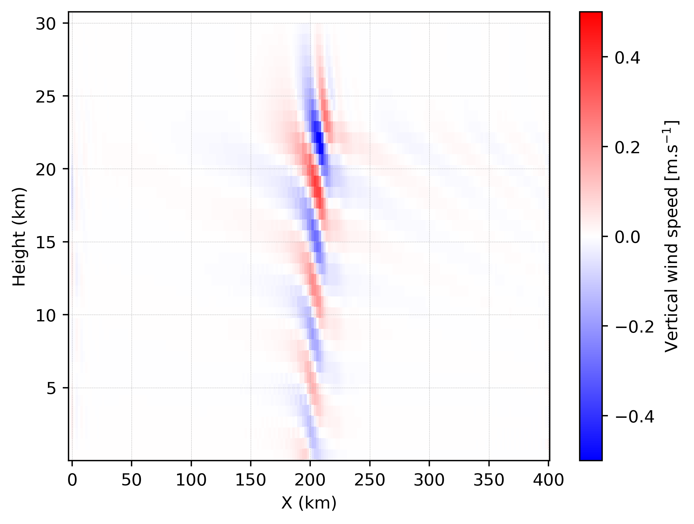
Example of 2D simulation output. Vertical wind velocity along cross section.
Tip
See the python script used to plot this figure:
#!/usr/bin/python
# -*- coding: utf-8 -*-

# ~~~~~~~~~~~~~~~~~~~~~~~~~~~~~~~~~~~~~~~~~~~~~~~~~~~~~~~~~
import numpy as np
import netCDF4
import matplotlib.pyplot as plt
# ~~~~~~~~~~~~~~~~~~~~~~~~~~~~~~~~~~~~~~~~~~~~~~~~~~~~~~~~~

# #########################################################
# ###           To be defined by user                   ###
# #########################################################

cfg_file_name = 'EXP01.1.SEG01.001.nc'

# #########################################################

# ------------------------------------------------------
#   Read netcdf file and variables
# ------------------------------------------------------

file_MNH     = netCDF4.Dataset(cfg_file_name)

xhat_MNH     = file_MNH['XHAT']
levels_MNH   = file_MNH['level_w'][1:]
x_MNH, z_MNH = np.meshgrid(xhat_MNH, levels_MNH)

zs_MNH       = file_MNH['ZS']
ztop_MNH     = 30000.0
wwnd_MNH     = file_MNH['WT'][0,1:,:]

# ------------------------------------------------------
#   Convert xhat, yhat, zs to alt
# ------------------------------------------------------

altitude = np.zeros((len(levels_MNH),len(xhat_MNH)))

for ind_i in range(len(xhat_MNH)):
  for ind_k in range(len(levels_MNH)):
    altitude[ind_k, ind_i] = zs_MNH[ind_i] + levels_MNH[ind_k] * ((ztop_MNH - zs_MNH[ind_i]) / ztop_MNH)

# ------------------------------------------------------
#   Quick plot
# ------------------------------------------------------

plt.pcolormesh(x_MNH[:,:]/1000.0, (altitude[:,:]+750.0/2.0)/1000.0, wwnd_MNH[:,:], vmin=-0.5, vmax=0.5, shading="auto", cmap="bwr")

# ------------------------------------------------------
#   Some adjustments to the plot
# ------------------------------------------------------

plt.grid(True, linestyle='--', linewidth=0.2)

cbar=plt.colorbar()
cbar.set_label(r"Vertical wind speed [m.s$^{-1}$]")

plt.xlabel("X (km)")
plt.ylabel("Height (km)")

plt.savefig('2D_orographic_wave.png', bbox_inches='tight', dpi=400)
This file is located here :
MNH-V6-1-0/examples/tutorials/ideal_cases/2D/003_python/
Other examples
You can find other 2D simulation examples in Namelist catalogue section.