Grid-nesting with 2 domains initialized and forced by ERA5
To perform a 3D Meso-NH simulation with real initial and surface conditions and two grid nested domains, you need to prepare the physiographic data for both domains, prepare the initial and lateral boundary conditions and run the model using the PREP_PGD, PREP_NEST_PGD, PREP_REAL_CASE, SPAWNING and MESONH executables respectively. In this example you will also use the DIAG program to calculate diagnostics after the simulation. These steps are described in the following sections:
Warning
This kind of simulation is parallelized and can be run with more than 1 core.
Note
You can find all the namelists presented in this section as well as the scripts here:
MNH-V6-1-0/examples/tutorials/real_cases/1domain_from_ERA5/
001_prep_pgd_d1 : directory to prepare the physiographic data
002_prep_pgd_d2 : directory to prepare the physiographic data
003_prep_nest_pgd_d1_and_d2 : directory to nest the physiographic data
004_prep_real_case_d1 : directory to prepare the initial condition for domain 1
005_spawning_d1_to_d2 : directory to spawn the domain 1 into domain 2
006_prep_real_case_d2 : directory to prepare the initial condition for domain 2
007_mesonh_d1_and_d2 : directory to run the model
008_diag_d1 : directory to calculate diagnostics after the simulation for domain 1
009_diag_d2 : directory to calculate diagnostics after the simulation for domain 2
010_python_d1_and_d2 : directory to plot the figure
The different steps must be performed in the order indicated by the directory numbers.
Prepare the physiographic data for domain 1 (PREP_PGD)
To create the physiographic file for domain 1 you have to use PREP_PGD program. This program reads a file called PRE_PGD1.nam defining the characteristics of the simulation.
Tip
To see all the namelists you can use in the PREP_PGD program or to obtain information about namelists, please go here.
In the PRE_PGD1.nam file, we recommend to have the following minimum informations and namelists:
The name of the NetCDF file you will create with the PREP_PGD program (without the extension) in NAM_PGDFILE namelist:
&NAM_PGDFILE CPGDFILE = "PGD_D1" /
Note
In this example, you will create a NetCDF file
PGD_D1.nccorresponding to surface boundary conditions files.The kind of desired projection you will use in NAM_PGD_GRID namelist:
&NAM_PGD_GRID CGRID = "CONF PROJ" /
Note
In this example, you will use conformal projection and you also need to define charastetics of this projection filling NAM_CONF_PROJ and NAM_CONF_PROJ_GRID namelists.
The characteristic of the conformal projection in NAM_CONF_PROJ namelist:
&NAM_CONF_PROJ XLAT0 = 43.604,
               XLON0 = 1.444,
               XRPK  = 0.,
               XBETA = 0. /
The characteristic of the conformal projection grid in NAM_CONF_PROJ_GRID namelist:
&NAM_CONF_PROJ_GRID XLATCEN = 43.604,
                    XLONCEN = 1.444,
                    NIMAX   = 50,
                    NJMAX   = 50,
                    XDX     = 10000.,
                    XDY     = 10000. /
Note
In this example, you will use a grid of 50x50 horizontal grid points, with a horizontal resolution of 10 km and the domain will be centered in Toulouse (lon=43.604, lat=1.444).
The kind of cover database you want to use in NAM_COVER namelist:
&NAM_COVER YCOVER         = "ECOCLIMAP_v2.0",
           YCOVERFILETYPE = "DIRECT" /
Note
In this example, you will use ECOCLIMAP_v2.0 database with more than 200 covers at 1 km horizontal resolution. Other database can be found here.
The kind of orography database you want to use in NAM_ZS namelist:
&NAM_ZS YZS         = "gtopo30",
        YZSFILETYPE = "DIRECT" /
Note
In this example, you will use gtopo30 database at approximately 1 km horizontal resolution. Other database can be found here.
The kind of clay and sand database you want to use in NAM_ISBA namelist:
&NAM_ISBA YCLAY         = "CLAY_HWSD_MOY",
          YCLAYFILETYPE = "DIRECT",
          YSAND         = "SAND_HWSD_MOY",
          YSANDFILETYPE = "DIRECT" /
Note
In this example, you will use CLAY_HWSD_MOY and SAND_HWSD_MOY database at 1 km horizontal resolution. Other database can be found here.
Tip
See the full PRE_PGD1.nam file:
&NAM_PGDFILE CPGDFILE = "PGD" /

&NAM_PGD_GRID CGRID = "CONF PROJ" /

&NAM_CONF_PROJ XLAT0 = 43.604,
               XLON0 = 1.444,
               XRPK  = 0.,
               XBETA = 0. /

&NAM_CONF_PROJ_GRID XLATCEN = 43.604,
                    XLONCEN = 1.444,
                    NIMAX   = 50,
                    NJMAX   = 50,
                    XDX     = 10000.,
                    XDY     = 10000. /

&NAM_COVER YCOVER         = "ECOCLIMAP_v2.0",
           YCOVERFILETYPE = "DIRECT" /

&NAM_ZS YZS         = "gtopo30",
        YZSFILETYPE = "DIRECT" /

&NAM_ISBA YCLAY         = "CLAY_HWSD_MOY",
          YCLAYFILETYPE = "DIRECT",
          YSAND         = "SAND_HWSD_MOY",
          YSANDFILETYPE = "DIRECT" /
This file is located here :
MNH-V6-1-0/examples/tutorials/real_cases/2domains_from_ERA5/001_prep_pgd_d1/.
You can launch PREP_PGD program using run_prep_pgd.sh script (execution takes less than 4 s):
cd MNH-V6-1-0/examples/tutorials/real_cases/2domains_from_ERA5/001_prep_pgd_d1/
./run_prep_pgd.sh
At the end of the PREP_PGD execution, you need to have following files:
your_run_directory/
PRE_PGD1.nam : The file you’ve created from this example
PGD_D1.nc : The NetCDF part of the physiographic data file
OUTPUT_LISTING0 : File containing debug informations
Tip
To verify that the program has been executed correctly, you should see the following lines at the end of the OUTPUT_LISTING0 file:
***************************
* PREP_PGD ends correctly *
***************************
Prepare the physiographic data for domain 2 (PREP_PGD)
To create the physiographic file for domain 2 you have to use PREP_PGD program. This program reads a file called PRE_PGD1.nam defining the characteristics of the simulation.
Tip
To see all the namelists you can use in the PREP_PGD program or to obtain information about namelists, please go here.
In the PRE_PGD1.nam file, we recommend to have the following minimum informations and namelists:
The name of the NetCDF file you will create with the PREP_PGD program (without the extension) in NAM_PGDFILE namelist:
&NAM_PGDFILE CPGDFILE = "PGD_D2" /
Note
In this example, you will create a NetCDF file
PGD_D2.nccorresponding to surface boundary conditions files.The kind of desired projection you will use in NAM_PGD_GRID namelist:
&NAM_PGD_GRID YINIFILE     = "PGD_D1",
              YINIFILETYPE = "MESONH" /
Note
In this example, you will create the domain 2 from the domain 1.
The position of the domain 2 inside the domain 1 in NAM_INIFILE_CONF_PROJ namelist:
&NAM_INIFILE_CONF_PROJ IXOR     = 20,
                       IYOR     = 20,
                       IXSIZE   = 12,
                       IYSIZE   = 12,
                       IDXRATIO = 4,
                       IDYRATIO = 4 /
Note
In this example, domain 2 will have 48x48 horizontal grid points and the bottom left corner of the domain is located at the 20,20 domain 1 grid point.
The kind of cover database you want to use in NAM_COVER namelist:
&NAM_COVER YCOVER         = "ECOCLIMAP_v2.0",
           YCOVERFILETYPE = "DIRECT" /
Note
In this example, you will use ECOCLIMAP_v2.0 database with more than 200 covers at 1 km horizontal resolution. Other database can be found here.
The kind of orography database you want to use in NAM_ZS namelist:
&NAM_ZS YZS         = "gtopo30",
        YZSFILETYPE = "DIRECT" /
Note
In this example, you will use gtopo30 database at approximately 1 km horizontal resolution. Other database can be found here.
The kind of clay and sand database you want to use in NAM_ISBA namelist:
&NAM_ISBA YCLAY         = "CLAY_HWSD_MOY",
          YCLAYFILETYPE = "DIRECT",
          YSAND         = "SAND_HWSD_MOY",
          YSANDFILETYPE = "DIRECT" /
Note
In this example, you will use CLAY_HWSD_MOY and SAND_HWSD_MOY database at 1 km horizontal resolution. Other database can be found here.
Tip
See the full PRE_PGD1.nam file:
&NAM_PGD_GRID YINIFILE     = "PGD_D1",
              YINIFILETYPE = "MESONH" /

&NAM_PGDFILE CPGDFILE = "PGD_D2" /

&NAM_INIFILE_CONF_PROJ IXOR     = 20,
                       IYOR     = 20,
                       IXSIZE   = 12,
                       IYSIZE   = 12,
                       IDXRATIO = 4,
                       IDYRATIO = 4 /

 &NAM_COVER YCOVER         = "ECOCLIMAP_v2.0",
            YCOVERFILETYPE = "DIRECT" /

 &NAM_ZS YZS         = "gtopo30",
         YZSFILETYPE = "DIRECT" /

 &NAM_ISBA YCLAY         = "CLAY_HWSD_MOY",
           YCLAYFILETYPE = "DIRECT",
           YSAND         = "SAND_HWSD_MOY",
           YSANDFILETYPE = "DIRECT" /
This file is located here :
MNH-V6-1-0/examples/tutorials/real_cases/2domains_from_ERA5/001_prep_pgd_d2/.
You can launch PREP_PGD program using run_prep_pgd.sh script (execution takes less than 4 s):
cd MNH-V6-1-0/examples/tutorials/real_cases/2domains_from_ERA5/001_prep_pgd_d2/
./run_prep_pgd.sh
At the end of the PREP_PGD execution, you need to have following files:
your_run_directory/
PRE_PGD1.nam : The file you’ve created from this example
PGD_D1.nc : The NetCDF part of the physiographic data file for domain 1
PGD_D2.nc : The NetCDF part of the physiographic data file for domain 2
OUTPUT_LISTING0 : File containing debug informations
Tip
To verify that the program has been executed correctly, you should see the following lines at the end of the OUTPUT_LISTING0 file:
***************************
* PREP_PGD ends correctly *
***************************
Make domains consistent (PREP_NEST_PGD)
To make domains consistents, you have to use PREP_NEST_PGD program. This program reads a file called PRE_NEST_PGD1.nam defining the characteristics of the simulation.
Tip
To see all the namelists you can use in the PREP_NEST_PGD program or to obtain information about namelists, please go here.
In the PRE_NEST_PGD1.nam file, we recommend to have the following minimum informations and namelists:
The name of the domain 1 in NAM_PGD1 namelist:
&NAM_PGD1 YPGD1 = "PGD_D1" /
The name of the domain 2 and its relation with domain 1 in NAM_PGD2 namelist:
&NAM_PGD2 YPGD2 = "PGD_D2", IDAD = 1 /
The name of the file you will create in NAM_NEST_PGD namelist:
&NAM_NEST_PGD YNEST="" /
Note
In this example, files created with prep_nest_pgd will have the name
PGD_D1.nest.ncandPGD_D2.nest.nc.
Tip
See the full PRE_NEST_PGD1.nam file:
&NAM_PGD1 YPGD1 = "PGD_D1" /

&NAM_PGD2 YPGD2 = "PGD_D2", IDAD = 1 /

&NAM_NEST_PGD YNEST="" /
This file is located here :
MNH-V6-1-0/examples/tutorials/real_cases/2domains_from_ERA5/003_prep_nest_pgd_d1_and_d2/.
You can launch PREP_NEST_PGD program using run_prep_nest_pgd.sh script (execution takes less than 4 s):
cd MNH-V6-1-0/examples/tutorials/real_cases/2domains_from_ERA5/003_prep_nest_pgd_d1_and_d2/
./run_prep_nest_pgd.sh
At the end of the PREP_NEST_PGD execution, you need to have following files:
your_run_directory/
PRE_NEST_PGD1.nam : The file you’ve created from this example
PGD_D1.nc : The NetCDF part of the physiographic data file of domain 1
PGD_D2.nc : The NetCDF part of the physiographic data file of domain 2
PGD_D1.nest.nc : The NetCDF part of the physiographic data file of domain 1, consitent with domain 2
PGD_D2.nest.nc : The NetCDF part of the physiographic data file of domain 2, consitent with domain 1
OUTPUT_LISTING0 : File containing debug informations
OUTPUT_LISTING1 : File containing debug informations
OUTPUT_LISTING2 : File containing debug informations
Tip
To verify that the program has been executed correctly, you should see the following lines at the end of the OUTPUT_LISTING0 file:
************************************************
* PREP_NEST_PGD: PREP_NEST_PGD ends correctly. *
************************************************
Prepare the initial and lateral boundary conditions for domain 1 (PREP_REAL_CASE)
To create the initial and lateral boundary condition files for a real case Meso-NH simulation you have to use PREP_REAL_CASE program. This program reads a file called PRE_REAL1.nam defining the characteristics of the simulation.
Tip
To see all the namelists you can use in the PREP_REAL_CASE program or to obtain information about namelists, please go here.
Note
Before using PREP_REAL_CASE program to create initial and lateral boundary condition files for Meso-NH, you need to extract three dimensional Initialization of atmospheric and surface data. In this example, you have to extract ERA5 data. At the end of the extraction you need to have the two grib files era5.20251113.18 and era5.20251113.18.
In the PRE_REAL1.nam file, we recommend to have the following minimum informations and namelists:
The information about PGD file created in previous section in NAM_FILE_NAMES namelist:
&NAM_FILE_NAMES HPGDFILE     = "PGD_D1.nest",
                HATMFILE     = "era5.YEARMONTHDAY.HOUR",
                HATMFILETYPE = "GRIBEX",
                CINIFILE     = "ERA5.D1.YEARMONTHDAY.HOUR" /
Note
You will physiographic data file created in the previous step.
You need to run PREP_REAL_CASE program twice, replacing YEARMONTHDAY.HOUR with the correct dates of the grib files (20251113.18 and 20251113.19). The first file created with PREP_REAL_CASE program (
CINIFILE) will correspond to the initial condition and the second to the lateral boundary condition.
The vertical grid discretisation in NAM_VER_GRID namelist:
&NAM_VER_GRID NKMAX        = 30,
              YZGRID_TYPE  = "FUNCTN",
              ZDZGRD       = 100.,
              ZDZTOP       = 3000.,
              ZZMAX_STRGRD = 1500.,
              ZSTRGRD      = 10.,
              ZSTRTOP      = 15. /
Note
In this example, you will use 30 vertical grid points with a vertical resolution of 100 m close to the ground and a stretching until the top of the domain with a maximum grid spacing of 3000 m.
Tip
See the full PRE_REAL1.nam file:
&NAM_FILE_NAMES HPGDFILE     = "PGD_D1.nest",
                HATMFILE     = "era5.YEARMONTHDAY.HOUR",
                HATMFILETYPE = "GRIBEX",
                CINIFILE     = "ERA5.D1.YEARMONTHDAY.HOUR" /

&NAM_VER_GRID NKMAX        = 30,
              YZGRID_TYPE  = "FUNCTN",
              ZDZGRD       = 100.,
              ZDZTOP       = 3000.,
              ZZMAX_STRGRD = 1500.,
              ZSTRGRD      = 10.,
              ZSTRTOP      = 15. /
This file is located here :
MNH-V6-1-0/examples/tutorials/real_cases/2domains_from_ERA5/004_prep_real_case_d1/
You can launch PREP_REAL_CASE program using run_prep_real_case.sh script (execution takes less than 4 s):
cd MNH-V6-1-0/examples/tutorials/real_cases/2domains_from_ERA5/004_prep_real_case_d1/
./run_prep_real_case.sh
At the end of the PREP_IDEAL_CASE execution, you need to have following files:
your_run_directory/
PRE_REAL1.nam : The file you’ve created from this example
ERA5.D1.20251113.18.des : The descriptive part of the initial condition file
ERA5.D1.20251113.18.nc : The NetCDF part of the initial condition file
ERA5.D1.20251113.19.des : The descriptive part of the lateral boundary condition file
ERA5.D1.20251113.19.nc : The NetCDF part of the lateral boundary condition file
PGD_D1.nest.nc : The NetCDF part of the physiographic data file
OUTPUT_LISTING0 : File containing debug informations
Tip
To verify that the program has been executed correctly, you should see the following lines at the end of the OUTPUT_LISTING1 file:
****************************************************
* PREP_REAL_CASE: PREP_REAL_CASE ENDS CORRECTLY. *
****************************************************
Interopolate horizontally domain 1 to domain 2 (SPAWNING)
To interpolate horizontally the fields from domain 1 to domain 2 you have to use SPAWNING program. This program reads a file called SPAWN1.nam defining the characteristics of the simulation.
Tip
To see all the namelists you can use in the SPAWNING program or to obtain information about namelists, please go here.
In the SPAWN1.nam file, we recommend to have the following minimum informations and namelists:
The information about files created in previous section in NAM_LUNIT2_SPA namelist:
&NAM_LUNIT2_SPA CINIFILE    = "ERA5.D1.20251113.18",
                CINIFILEPGD = "PGD_D1.nest",
                YDOMAIN     = "PGD_D2.nest",
                YSPANBR     = "" /
Tip
See the full SPAWN1.nam file:
&NAM_LUNIT2_SPA CINIFILE    = "ERA5.D1.20251113.18",
                CINIFILEPGD = "PGD_D1.nest",
                YDOMAIN     = "PGD_D2.nest",
                YSPANBR     = "" /
This file is located here :
MNH-V6-1-0/examples/tutorials/real_cases/2domains_from_ERA5/005_spawning_d1_to_d2/
You can launch SPAWNING program using run_spawning.sh script (execution takes less than 4 s):
cd MNH-V6-1-0/examples/tutorials/real_cases/2domains_from_ERA5/005_spawning_d1_to_d2/
./run_spawning.sh
At the end of the SPAWNING execution, you need to have following files:
your_run_directory/
SPAWN1.nam : The file you’ve created from this example
ERA5.D1.20251113.18.des : The descriptive part of the initial condition file
ERA5.D1.20251113.18.nc : The NetCDF part of the initial condition file
PGD_D1.nest.nc : The NetCDF part of the physiographic data file for domain 1
PGD_D2.nest.nc : The NetCDF part of the physiographic data file for domain 2
OUTPUT_LISTING0 : File containing debug informations
OUTPUT_LISTING1 : File containing debug informations
OUTPUT_LISTING2 : File containing debug informations
Tip
To verify that the program has been executed correctly, you should see the following lines at the end of the OUTPUT_LISTING2 file:
SPAWN_MODEL2: SPAWN_MODEL2 ENDS CORRECTLY.
Prepare the initial and lateral boundary conditions for domain 2 (PREP_REAL_CASE)
To create the initial condition files for domain 2 you have to use PREP_REAL_CASE program. This program reads a file called PRE_REAL1.nam defining the characteristics of the simulation.
Tip
To see all the namelists you can use in the PREP_REAL_CASE program or to obtain information about namelists, please go here.
In the PRE_REAL1.nam file, we recommend to have the following minimum informations and namelists:
The information about input atmospheric file created in previous section in NAM_FILE_NAMES namelist:
&NAM_FILE_NAMES HATMFILE     = "ERA5.D1.20251113.18.spa",
                HATMFILETYPE = "MESONH",
                HPGDFILE     = "PGD_D2.nest",
                CINIFILE     = "ERA5.D2.20251113.18" /
The information about input surface file in NAM_PREP_SURF_ATM namelist:
&NAM_PREP_SURF_ATM CFILE     = "ERA5.D1.20251113.18",
                   CFILEPGD  = "PGD_D1.nest",
                   CFILETYPE = "MESONH" /
Tip
See the full PRE_REAL1.nam file:
 &NAM_FILE_NAMES HATMFILE     = "ERA5.D1.20251113.18.spa",
                 HATMFILETYPE = "MESONH",
                 HPGDFILE     = "PGD_D2.nest",
                 CINIFILE     = "ERA5.D2.20251113.18" /

&NAM_PREP_SURF_ATM CFILE     = "ERA5.D1.20251113.18",
                   CFILEPGD  = "PGD_D1.nest",
                   CFILETYPE = "MESONH" /
This file is located here :
MNH-V6-1-0/examples/tutorials/real_cases/2domains_from_ERA5/006_prep_real_case_d2/
You can launch PREP_REAL_CASE program using run_prep_real_case.sh script (execution takes less than 4 s):
cd MNH-V6-1-0/examples/tutorials/real_cases/2domains_from_ERA5/006_prep_real_case_d2/
./run_prep_real_case.sh
At the end of the PREP_REAL_CASE execution, you need to have following files:
your_run_directory/
PRE_REAL1.nam : The file you’ve created from this example
ERA5.D1.20251113.18spa.des : The descriptive part of the initial atmospheric condition file for domain 1
ERA5.D1.20251113.18spa.nc : The NetCDF part of the initial atmospheric condition file for domain 1
ERA5.D1.20251113.18.des : The descriptive part of the initial surface condition file for domain 1
ERA5.D1.20251113.18.nc : The NetCDF part of the initial surface condition file for domain 1
ERA5.D2.20251113.18.des : The descriptive part of the initial condition file for domain 2
ERA5.D2.20251113.18.nc : The NetCDF part of the initial condition file for domain 2
PGD_D1.nest.nc : The NetCDF part of the physiographic data file for domain 1
PGD_D2.nest.nc : The NetCDF part of the physiographic data file for domain 2
OUTPUT_LISTING0 : File containing debug informations
OUTPUT_LISTING1 : File containing debug informations
Tip
To verify that the program has been executed correctly, you should see the following lines at the end of the OUTPUT_LISTING1 file:
****************************************************
* PREP_REAL_CASE: PREP_REAL_CASE ENDS CORRECTLY. *
****************************************************
Launch the simulation (MESONH)
To launch the Meso-NH simulation on two domains you have to use MESONH program. This program reads two files called EXSEG1.nam and EXSEG2.nam defining the characteristics of the two simulated domains.
Tip
To see all the namelists you can use in the MESONH program or to obtain information about namelists, please go here.
In the EXSEG1.nam file, we recommend to have the following minimum informations and namelists:
The name of the NetCDF files created by the PREP_PGD and PREP_REAL_CASE program in NAM_LUNITn namelist:
&NAM_LUNITn CINIFILE    = "ERA5.D1.20251113.18",
            CINIFILEPGD = "PGD_D1.nest",
            CCPLFILE(1) = "ERA5.D1.20251113.19" /
The name of the experiment and segment and the configuration of the simulation in NAM_CONF namelist:
&NAM_CONF CCONF   = "START",
          NMODEL  = 2,
          CEXP    = "EXP01",
          CSEG    = "SEG01" /
Note
In this example, you will do a START from ERA5 data directly. Other possibility is to do a RESTArt from a previous segment.
Simulation file names will be of the type
CEXP.1.CSEG.XXX.nc.
The kind of dependance between the two domains in NAM_NESTING namelist:
&NAM_NESTING NDAD(2) = 1, NDTRATIO(2) = 4, XWAY(2) = 2. /
Note
In this example, domain 1 and domain 2 are coupled in two-way nesting and time step of domain 2 is 4 times smaller than the one used in domain 1.
The simulated length (in s), the top absorbing layer coefficient and the activation of numerical diffusion in NAM_DYN namelist :
&NAM_DYN XSEGLEN  = 600.,
         LNUMDIFU = .TRUE.,
         XALKTOP  = 0.01,
         XALZBOT  = 14000. /
The backup output writing period in NAM_BACKUP namelist:
&NAM_BACKUP XBAK_TIME(1,1) = 600.0 /
The time step, pressure solver option and the activation of the top absorbing layer in NAM_DYNn namelist:
&NAM_DYNn XTSTEP         = 10.,
          CPRESOPT       = "CRESI",
          LHORELAX_UVWTH = .TRUE.,
          LHORELAX_RV    = .TRUE.,
          LVE_RELAX      = .TRUE.,
          NRIMX          = 5,
          NRIMY          = 5,
          XT4DIFU        = 1800. /
The temporal and advection schemes in NAM_ADVn namelist:
&NAM_ADVn CTEMP_SCHEME    = "RKC4",
          CUVW_ADV_SCHEME = "CEN4TH",
          CMET_ADV_SCHEME = "PPM_01" /
The lateral boundary condition options NAM_LBCn namelist:
&NAM_LBCn CLBCX = 2*"OPEN",
          CLBCY = 2*"OPEN" /
Note
In this example you will use open boundary condition in i and j directions.
The physical parametrization options in NAM_PARAMn namelist:
&NAM_PARAMn CTURB  = "TKEL",
            CRAD   = "ECMW",
            CCLOUD = "ICE3",
            CSCONV = "EDKF",
            CDCONV = "KAFR" /
Note
In this example, you will use turbulence, radiative, miscrophysics, shallow and deep convection parametrizations.
The radiative parametrization options in NAM_PARAM_RADn namelist:
&NAM_PARAM_RADn XDTRAD        = 300.,
                XDTRAD_CLONLY = 300. /
The convective parametrization options in NAM_PARAM_KAFRn namelist:
&NAM_PARAM_KAFRn XDTCONV = 300. /
The turbulent parametrization options in NAM_TURBn namelist:
&NAM_TURBn CTURBLEN = "BL89",
           CTURBDIM = "1DIM" /
Tip
See the full EXSEG1.nam file:
&NAM_LUNITn CINIFILE    = "ERA5.D1.20251113.18",
            CINIFILEPGD = "PGD_D1.nest",
            CCPLFILE(1) = "ERA5.D1.20251113.19" /

&NAM_CONF CCONF   = "START",
          NMODEL  = 2,
          CEXP    = "EXP01",
          CSEG    = "SEG01" /

&NAM_NESTING NDAD(2) = 1, NDTRATIO(2) = 4, XWAY(2) = 2. /

&NAM_DYN XSEGLEN  = 600.,
         LNUMDIFU = .TRUE.,
         XALKTOP  = 0.01,
         XALZBOT  = 14000. /

&NAM_BACKUP XBAK_TIME(1,1) = 600. /

&NAM_DYNn XTSTEP         = 10.,
          CPRESOPT       = "CRESI",
          LHORELAX_UVWTH = .TRUE.,
          LHORELAX_RV    = .TRUE.,
          LVE_RELAX      = .TRUE.,
          NRIMX          = 5,
          NRIMY          = 5,
          XT4DIFU        = 1800. /

&NAM_ADVn CTEMP_SCHEME    = "RKC4",
          CUVW_ADV_SCHEME = "CEN4TH",
          CMET_ADV_SCHEME = "PPM_01" /

&NAM_LBCn CLBCX = 2*"OPEN",
          CLBCY = 2*"OPEN" /

&NAM_PARAMn CTURB  = "TKEL",
            CRAD   = "ECMW",
            CCLOUD = "ICE3",
            CSCONV = "EDKF",
            CDCONV = "KAFR" /

&NAM_PARAM_RADn XDTRAD        = 300.,
                XDTRAD_CLONLY = 300. /

&NAM_PARAM_KAFRn XDTCONV = 300. /

&NAM_TURBn CTURBLEN = "BL89",
           CTURBDIM = "1DIM" /
This file is located here :
MNH-V6-1-0/examples/tutorials/real_cases/2domains_from_ERA5/007_mesonh_d1_and_d2/
For domain 2, we recommend to have the following minimum informations and namelists in EXSEG2.nam file:
The name of the NetCDF files created by the PREP_PGD and PREP_REAL_CASE program in NAM_LUNITn namelist:
&NAM_LUNITn CINIFILE    = "ERA5.D2.20251113.18",
            CINIFILEPGD = "PGD_D2.nest" /
The time step, pressure solver option and the activation of the top absorbing layer in NAM_DYNn namelist:
&NAM_DYNn LVE_RELAX      = .TRUE.,
          XT4DIFU        = 1800. /
The temporal and advection schemes in NAM_ADVn namelist:
&NAM_ADVn CTEMP_SCHEME    = "RKC4",
          CUVW_ADV_SCHEME = "CEN4TH",
          CMET_ADV_SCHEME = "PPM_01" /
The lateral boundary condition options NAM_LBCn namelist:
&NAM_LBCn CLBCX = 2*"OPEN",
          CLBCY = 2*"OPEN" /
Note
In this example you will use open boundary condition in i and j directions.
The physical parametrization options in NAM_PARAMn namelist:
&NAM_PARAMn CTURB  = "TKEL",
            CRAD   = "ECMW",
            CCLOUD = "ICE3",
            CSCONV = "EDKF",
            CDCONV = "NONE" /
Note
In this example, you will use turbulence, radiative, miscrophysics and shallow convection parametrizations.
The radiative parametrization options in NAM_PARAM_RADn namelist:
&NAM_PARAM_RADn XDTRAD        = 300.,
                XDTRAD_CLONLY = 300. /
The convective parametrization options in NAM_PARAM_KAFRn namelist:
&NAM_PARAM_KAFRn XDTCONV = 300. /
The turbulent parametrization options in NAM_TURBn namelist:
&NAM_TURBn CTURBLEN = "BL89",
           CTURBDIM = "1DIM" /
Tip
See the full EXSEG2.nam file:
&NAM_LUNITn CINIFILE    = "ERA5.D2.20251113.18",
            CINIFILEPGD = "PGD_D2.nest" /

&NAM_DYNn LVE_RELAX      = .TRUE.,
          XT4DIFU        = 1800. /

&NAM_ADVn CTEMP_SCHEME    = "RKC4",
          CUVW_ADV_SCHEME = "CEN4TH",
          CMET_ADV_SCHEME = "PPM_01" /

&NAM_LBCn CLBCX = 2*"OPEN",
          CLBCY = 2*"OPEN" /

&NAM_PARAMn CTURB  = "TKEL",
            CRAD   = "ECMW",
            CCLOUD = "ICE3",
            CSCONV = "EDKF",
            CDCONV = "NONE" /

&NAM_PARAM_RADn XDTRAD        = 300.,
                XDTRAD_CLONLY = 300. /

&NAM_PARAM_KAFRn XDTCONV = 300. /

&NAM_TURBn CTURBLEN = "BL89",
           CTURBDIM = "1DIM" /
This file is located here :
MNH-V6-1-0/examples/tutorials/real_cases/2domains_from_ERA5/007_mesonh_d1_and_d2/
You can launch MESONH program using run_mesonh.sh script (execution takes less than 50 s on 2 cores):
cd MNH-V6-1-0/examples/tutorials/real_cases/2domains_from_ERA5/007_mesonh_d1_and_d2/
./run_mesonh.sh
At the end of the MESONH execution, you need to have following files:
your_run_directory/
PGD.nc : The NetCDF part of the physiographic data file
ERA5.D1.20251113.18.des : The descriptive part of the initial condition file
ERA5.D1.20251113.18.nc : The NetCDF part of the initial condition file
ERA5.D2.20251113.18.des : The descriptive part of the initial condition file
ERA5.D2.20251113.18.nc : The NetCDF part of the initial condition file
ERA5.D1.20251113.19.des : The descriptive part of the lateral boundary condition file
ERA5.D1.20251113.19.nc : The NetCDF part of the lateral boundar condition file
EXSEG1.nam : The file you’ve created from this example
EXSEG2.nam : The file you’ve created from this example
EXP01.1.SEG01.000.des : The descriptive part of the simulated output file
EXP01.1.SEG01.000.nc : The NetCDF part of the simulated output file
EXP01.1.SEG01.001.des : The descriptive part of the simulated output file
EXP01.1.SEG01.001.nc : The NetCDF part of the simulated output file
EXP01.2.SEG01.000.des : The descriptive part of the simulated output file
EXP01.2.SEG01.000.nc : The NetCDF part of the simulated output file
EXP01.2.SEG01.001.des : The descriptive part of the simulated output file
EXP01.2.SEG01.001.nc : The NetCDF part of the simulated output file
OUTPUT_LISTING1 : File containing debug informations
OUTPUT_LISTING2 : File containing debug informations
Tip
The *.001.nc file contains NAM_BACKUP output. This file can be used to restart the simulation. It contains one time variables.
To verify that the program has been executed correctly, you should see the following lines at the end of the
OUTPUT_LISTING1andOUTPUT_LISTING2file:|++++++++++++++++++++++++++++++++++++++++++++++++++++++++++++++++++++++++++++++++++++++++++++++++++++| | MODEL1 | CPUTIME || 85.057| 42.528| 42.437| 42.620| 100.000| | MODEL1 | ELAPSED || 85.151| 42.576| 42.530| 42.621| 100.000| |++++++++++++++++++++++++++++++++++++++++++++++++++++++++++++++++++++++++++++++++++++++++++++++++++++| |++++++++++++++++++++++++++++++++++++++++++++++++++++++++++++++++++++++++++++++++++++++++++++++++++++| |++++++++++++++++++++++++++++++++++++++++++++++++++++++++++++++++++++++++++++++++++++++++++++++++++++| |====================================================================================================| | SECOND/STEP=61 | CPUTIME || 1.394| 0.697| 0.696| 0.699| 1.639| | SECOND/STEP=61 | ELAPSED || 1.396| 0.698| 0.697| 0.699| 1.639| |----------------------------------------------------------------------------------------------------| | MICROSEC/STP/PT=75000 | CPUTIME || 18.592| 9.296| 9.276| 9.316| 100.000| | MICROSEC/STP/PT=75000 | ELAPSED || 18.612| 9.306| 9.296| 9.316| 100.000| |====================================================================================================|
|++++++++++++++++++++++++++++++++++++++++++++++++++++++++++++++++++++++++++++++++++++++++++++++++++++|
| MODEL2                      | CPUTIME ||        257.616|   128.808|   128.713|   128.903|   100.000|
| MODEL2                      | ELAPSED ||        257.898|   128.949|   128.908|   128.990|   100.000|
|++++++++++++++++++++++++++++++++++++++++++++++++++++++++++++++++++++++++++++++++++++++++++++++++++++|
|++++++++++++++++++++++++++++++++++++++++++++++++++++++++++++++++++++++++++++++++++++++++++++++++++++|
|++++++++++++++++++++++++++++++++++++++++++++++++++++++++++++++++++++++++++++++++++++++++++++++++++++|
|====================================================================================================|
| SECOND/STEP=241             | CPUTIME ||          1.069|     0.534|     0.534|     0.535|     0.415|
| SECOND/STEP=241             | ELAPSED ||          1.070|     0.535|     0.535|     0.535|     0.415|
|----------------------------------------------------------------------------------------------------|
| MICROSEC/STP/PT=69120       | CPUTIME ||         15.465|     7.733|     7.727|     7.738|   100.000|
| MICROSEC/STP/PT=69120       | ELAPSED ||         15.482|     7.741|     7.739|     7.743|   100.000|
|====================================================================================================|
Compute diagnostics after the simulation (DIAG)
To compute diagnostics after a Meso-NH simulation you have to use DIAG program. This program reads a file called DIAG1.nam defining the characteristics of the diagnostics you want.
Tip
To see all the namelists you can use in the DIAG program or to obtain information about namelists, please go here.
In the DIAG1.nam file, we recommend to have the following minimum informations and namelists:
The name of input NetCDF files and the extension of the one created by the DIAG program in NAM_DIAG_FILE namelist:
&NAM_DIAG_FILE YINIFILE(1)    = "EXP01.1.SEG01.001",
               YINIFILEPGD(1) = "PGD",
               YSUFFIX        = "diag" /
Note
In this example, you will create a file called
EXP01.1.SEG01.001diag.nc.
The type of diag you want to perform in NAM_DIAG namelist :
&NAM_DIAG LISOAL    = .TRUE.,
          XISOAL(1) = 500.0 /
Note
In this example, you will interpolate some variables at a constant altitude of 500 m above sea level.
Tip
See the full DIAG1.nam file:
&NAM_DIAG_FILE YINIFILE(1)    = "EXP01.1.SEG01.001",
               YINIFILEPGD(1) = "PGD",
               YSUFFIX        = "diag" /

&NAM_DIAG LISOAL    = .TRUE.,
          XISOAL(1) = 500.0 /
This file is located here :
MNH-V6-1-0/examples/tutorials/real_cases/2domains_from_ERA5/008_diag_d1/
You can launch DIAG program using run_diag.sh script (execution takes less than 15 s):
cd MNH-V6-1-0/examples/tutorials/real_cases/2domains_from_ERA5/008_diag_d1/
./run_diag.sh
At the end of the DIAG execution, you need to have following files:
your_run_directory/
PGD.nc : The NetCDF part of the physiographic data file
DIAG1.nam : The file you’ve created from this example
EXP01.1.SEG01.001.des : The descriptive part of the simulated output file
EXP01.1.SEG01.001.nc : The NetCDF part of the simulated output file
EXP01.1.SEG01.001diag.nc : The NetCDF part of the diagnostic output file
OUTPUT_LISTING0 : File containing debug informations
OUTPUT_LISTING1 : File containing debug informations
Tip
To verify that the program has been executed correctly, you should see the following lines at the end of the OUTPUT_LISTING0 file:
***************************** **************
*            EXIT  DIAG CORRECTLY          *
**************************** ***************
Note
You have to compute diagnostic for both domains in MNH-V6-1-0/examples/tutorials/real_cases/2domains_from_ERA5/009_diag_d2/.
Plot results
The following figure shows an example of a graph that you can plot from the two domains simulation you just performed. It shows a classic episode of the Autan wind. Gray areas correspond to mountain higher than 500 m.
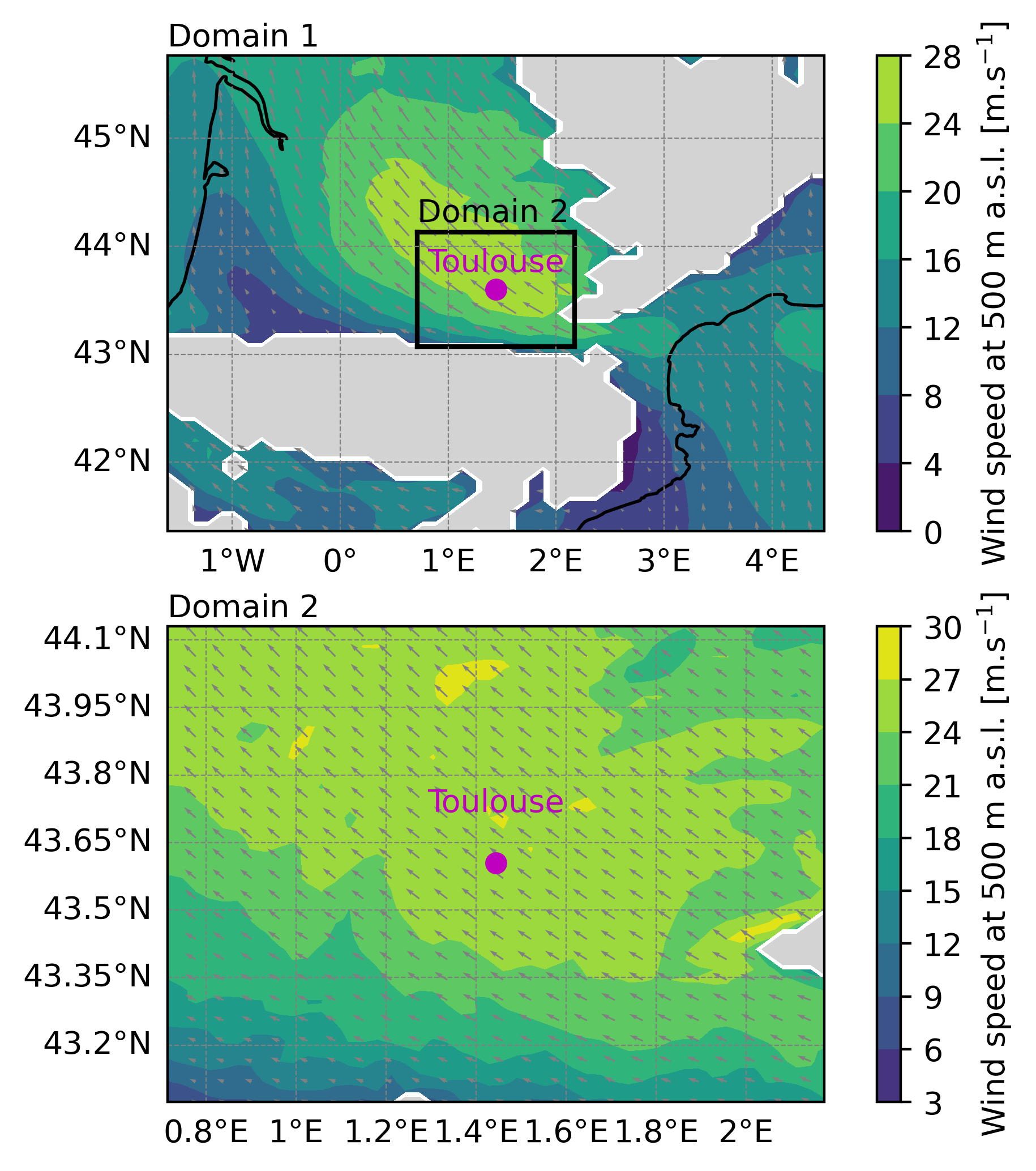
Example of the two domains case simulation output. Horizontal wind speed at 500 m a.s.l.
Tip
See the python script used to plot this figure:
#!/usr/bin/python
# -*- coding: utf-8 -*-

# ~~~~~~~~~~~~~~~~~~~~~~~~~~~~~~~~~~~~~~~~~~~~~~~~~~~~~~~~~
import numpy as np
import netCDF4
import matplotlib.pyplot as plt
import matplotlib.gridspec as gridspec
import cartopy.crs as ccrs
# ~~~~~~~~~~~~~~~~~~~~~~~~~~~~~~~~~~~~~~~~~~~~~~~~~~~~~~~~~

# #########################################################
# ###           To be defined by user                   ###
# #########################################################

cfg_file_name_d1 = 'EXP01.1.SEG01.001diag.nc'
cfg_file_name_d2 = 'EXP01.2.SEG01.001diag.nc'

# #########################################################

# ------------------------------------------------------
#   Read netcdf file and variables
# ------------------------------------------------------

file_MNH_d1 = netCDF4.Dataset(cfg_file_name_d1)
file_MNH_d2 = netCDF4.Dataset(cfg_file_name_d2)

lon_MNH_d1 = file_MNH_d1['LON'][1:-1,1:-1]
lat_MNH_d1 = file_MNH_d1['LAT'][1:-1,1:-1]

lon_MNH_d2 = file_MNH_d2['LON'][1:-1,1:-1]
lat_MNH_d2 = file_MNH_d2['LAT'][1:-1,1:-1]

uwnd_MNH_d1 = file_MNH_d1['ALT_U'][0,0,1:-1,1:-1]
vwnd_MNH_d1 = file_MNH_d1['ALT_V'][0,0,1:-1,1:-1]

uwnd_MNH_d2 = file_MNH_d2['ALT_U'][0,0,1:-1,1:-1]
vwnd_MNH_d2 = file_MNH_d2['ALT_V'][0,0,1:-1,1:-1]

mask_MNH_d1 = uwnd_MNH_d1 < -1000.0
mask_MNH_d2 = uwnd_MNH_d2 < -1000.0

uwnd_MNH_masked_d1 = np.ma.masked_where(mask_MNH_d1, uwnd_MNH_d1)
vwnd_MNH_masked_d1 = np.ma.masked_where(mask_MNH_d1, vwnd_MNH_d1)

uwnd_MNH_masked_d2 = np.ma.masked_where(mask_MNH_d2, uwnd_MNH_d2)
vwnd_MNH_masked_d2 = np.ma.masked_where(mask_MNH_d2, vwnd_MNH_d2)

wnd_MNH_masked_d1 = np.sqrt(uwnd_MNH_masked_d1**2.0+vwnd_MNH_masked_d1**2.0)
wnd_MNH_masked_d2 = np.sqrt(uwnd_MNH_masked_d2**2.0+vwnd_MNH_masked_d2**2.0)

lon_north_d2 = lon_MNH_d2[-1, :] ; lat_north_d2 = lat_MNH_d2[-1, :]
lon_south_d2 = lon_MNH_d2[ 0, :] ; lat_south_d2 = lat_MNH_d2[0 , :]
lon_west_d2  = lon_MNH_d2[: , 0] ; lat_west_d2  = lat_MNH_d2[: , 0]
lon_east_d2  = lon_MNH_d2[: ,-1] ; lat_east_d2  = lat_MNH_d2[: ,-1]

# ------------------------------------------------------
#   Quick plot
# ------------------------------------------------------

gs  = gridspec.GridSpec(2,1)
fig = plt.figure(figsize=(6, 6))
#ax  = plt.axes(projection=ccrs.PlateCarree())

# ------------------------------------------------------
#   Domain 1
# ------------------------------------------------------
ax0   = fig.add_subplot(gs[0,0], projection=ccrs.PlateCarree())
pmsh0 = ax0.contourf(lon_MNH_d1[:,:], lat_MNH_d1[:,:], wnd_MNH_masked_d1[:,:], vmin=0.0, vmax=30.0, shading="auto", cmap="viridis")
ctf0  = ax0.contourf(lon_MNH_d1[:,:], lat_MNH_d1[:,:], mask_MNH_d1[:,:], levels=[0.5, 1], colors='lightgray')
qvr0  = ax0.quiver(lon_MNH_d1[::2, ::2], lat_MNH_d1[::2, ::2], uwnd_MNH_masked_d1[::2, ::2], vwnd_MNH_masked_d1[::2, ::2], color="gray")

ax0.plot(lon_north_d2, lat_north_d2, 'k')
ax0.plot(lon_south_d2, lat_south_d2, 'k')
ax0.plot(lon_west_d2,   lat_west_d2, 'k')
ax0.plot(lon_east_d2,   lat_east_d2, 'k')

# ------------------------------------------------------
#   Domain 2
# ------------------------------------------------------
ax1   = fig.add_subplot(gs[1,0], projection=ccrs.PlateCarree())
pmsh1 = ax1.contourf(lon_MNH_d2[:,:], lat_MNH_d2[:,:], wnd_MNH_masked_d2[:,:], vmin=0.0, vmax=30.0, shading="auto", cmap="viridis")
ctf1  = ax1.contourf(lon_MNH_d2[:,:], lat_MNH_d2[:,:], mask_MNH_d2[:,:], levels=[0.5, 1], colors='lightgray')
qvr1  = ax1.quiver(lon_MNH_d2[::2, ::2], lat_MNH_d2[::2, ::2], uwnd_MNH_masked_d2[::2, ::2], vwnd_MNH_masked_d2[::2, ::2], color="gray")

# ------------------------------------------------------
#   Some adjustments to the plot
# ------------------------------------------------------
gl0 = ax0.gridlines(draw_labels=True, linewidth=0.4, color='gray', linestyle='--')
gl1 = ax1.gridlines(draw_labels=True, linewidth=0.4, color='gray', linestyle='--')

gl0.top_labels = False ; gl0.right_labels = False
gl1.top_labels = False ; gl1.right_labels = False

ax0.coastlines()
ax1.coastlines()

cbar0=plt.colorbar(pmsh0)#,shrink=0.59)
cbar0.set_label(r"Wind speed at 500 m a.s.l. [m.s$^{-1}$]")

cbar1=plt.colorbar(pmsh1)#,shrink=0.59)
cbar1.set_label(r"Wind speed at 500 m a.s.l. [m.s$^{-1}$]")

ax0.plot(1.444, 43.604, marker='o', color='m', markersize=6)
ax0.text(1.444, 43.604+0.1, "Toulouse", color='m', fontsize=10, ha='center', va='bottom')

ax1.plot(1.444, 43.604, marker='o', color='m', markersize=6)
ax1.text(1.444, 43.604+0.1, "Toulouse", color='m', fontsize=10, ha='center', va='bottom')

plt.text(0.0,1.02,r'Domain 1', transform = ax0.transAxes)
ax0.text(np.min(lon_north_d2),np.max(lat_north_d2)+0.1,r'Domain 2')#, transform = ax1.transAxes)
plt.text(0.0,1.02,r'Domain 2', transform = ax1.transAxes)

plt.savefig('two_domains_era5.png', bbox_inches='tight', dpi=400)
This file is located here :
MNH-V6-1-0/examples/tutorials/real_cases/2domains_from_ERA5/010_python_d1_and_d2/
Other examples
You can find multiple domains simulation examples in Namelist catalogue section.