How to ?
Compute altitude of vertical levels
Print the vertical grid computed from PREP_REAL_CASE and PRE_IDEAL_CASE namelist options. For that, you can copy and run the following python’s script :
# -*- coding: utf-8 -*-

KMAX=120 #nb levels
ZMAX=5000 #ZMAX_STRGRD
ZGRD=10 # mesh size at the ground ZGRD
ZTOP=300 # Mesh size at the top ZTOP
SGRD=4 # low level stretching SGRD
STOP=5 # top level stretching STOP

RZ=[0 for i in range(1,KMAX+1)]
RZ[1]=0.
RZ[2]=ZGRD

for i in range(2,KMAX-1):
  if RZ[i]<= ZMAX:
    RZ[i+1]=RZ[i] +(RZ[i]-RZ[i-1])* (1+SGRD/100)
  else:
    RZ[i+1]=RZ[i] +(RZ[i]-RZ[i-1])* (1+STOP/100)

  if (RZ[i+1]-RZ[i]) >=ZTOP:
    RZ[i+1]=RZ[i]+ZTOP

 print(RZ)
Suppress the orography
Use the following script to read and modify any .dir topography database (from SURFEX website) before ingesting the modified topography file at the PGD step.
#!/usr/bin/env python3
# -*- coding: utf-8 -*-
"""
CNRM, Université de Toulouse, Météo-France, CNRS, Toulouse, France
Created on 12 Avril 2020 - Marc Mandement - marc.mandement@meteo.fr
Script to modify the binary topography.dir file (tested on srtm_ne_250 and srtm_europe)
MODIFICATION
Q. Rodier 17/12/2020 : adapt to any topography .dir database.
"""

import matplotlib as mpl; mpl.use('Agg')
import matplotlib.pyplot as plt
import numpy as np
from mpl_toolkits.axes_grid1 import AxesGrid

def truncate_colormap(cmap, minval=0.0, maxval=1.0, n=100):
   n_cm = mpl.colors.LinearSegmentedColormap.from_list('trunc({n},{a:.2f},{b:.2f})'.format(n=cmap.name, a=minval, b=maxval),cmap(np.linspace(minval, maxval, n)))
   return n_cm

# Warning : the topography file are usually heavy and need > 4Go RAM memory
directory='/home/rodierq/RELIEF/' # Your directory
file=directory+'srtm_europe.dir'  # The topography file

with open(file, 'rb') as f:
   raw_data=np.fromfile(f,dtype='i2')

#Read the database
data=raw_data.reshape((18000,18000)) #This numbers must match the rows and cols written in the .hdr file
data=data[::-1,::] #Inverse coordinates Y X
modified_data=np.copy(data)

# Subset you are interested in (being plotted later), to decrease memory usage and plot
modified_data=data[3000:7000,5000:9000] #Here is an example of south-west France over the Pyrenees

#Initial data in the subdomain for plot
initial_data_sub=np.copy(modified_data)
#
#
# MODIFY YOUR OROGRAPHY HERE
#
#
modified_data[:750,:] = 250. #Example of erase the Pyrenees
#
#

# Plot before and after modification
cmap = truncate_colormap(plt.get_cmap('terrain'), 0.2, 1)
cmap.set_under('lightblue')

# Limit values of contour plot
vmin,vmax=0,2500

fig = plt.figure(figsize=(12,9))
ax = AxesGrid(fig, 111, nrows_ncols=(2,1),axes_pad=0.05,cbar_location="right",cbar_mode="single",cbar_size="4%",cbar_pad=0.4)

ax[0].contourf(initial_data_sub,np.linspace(vmin,vmax,41),cmap=cmap,vmin=vmin,vmax=vmax,extend='both')
bb=ax[1].contourf(modified_data,np.linspace(vmin,vmax,41),cmap=cmap,vmin=vmin,vmax=vmax,extend='both')
ax[0].set_title("Before and after modification",fontsize=25)
ax[0].tick_params(axis='both',labelsize=20) ; ax[1].tick_params(axis='both',labelsize=20)

#Colorbar
cbar=plt.colorbar(bb, cax = ax.cbar_axes[0])
cbar.ax.tick_params(labelsize=25)

fig.tight_layout()
fig.savefig(directory+"Orography.png")
plt.close()

#Write the modified orography
file_modified=directory+'srtm_europe_modif.dir'
raw_data.tofile(file_modified)
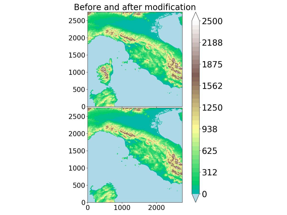
Example of removing Corsica within the srtm_ne_250 database
Test code’s reproducibility
(results independent of the number of MPI tasks)
The method consists of running simultaneously the same run with 2 different numbers of MPI tasks. The 2 runs exchange information to check that fields are equal.
For a MESONH execution :
In EXSEG1.nam, in NAM_CONF put LCHECK=.T.
Create a directory dir_clone_1proc on your run directory and copy run_mesonh_xyz_MPPDB
Copy mppdb.nam.ihm on your run directory and modify MPPDB_HOST by the name of your machine
Copy EXSEG1.nam to EXSEG1.nam.ihm, you can then launch run_mesonh_xyz_MPPDB and differences between the 2 runs will be printed.
For another step than the MESONH execution :
Instead of using LCHECK, you have to add check points in the source code by introducing USE MODE_MPPDB and calls to MPPDB_CHECK2D or MPPDB_CHECK3D. By example in ver_thermo.f90 :
CALL MPPDB_CHECK2D(PZSMT_LS,"ver_thermo:PZSMT_LS",PRECISION)
CALL MPPDB_CHECK3D(PZMASS_MX,"ver_thermo:PZMASS_MX",PRECISION)
then recompile your modified code, and then execute the steps 2 to 4 as previously after adapting to PREP_REAL_CASE or DIAG or …
run_mesonh_xyz_MPPDB script :
set -x
set -e
ln -fs ../001_prep_ideal_case/EI* .
ln -fs ../001_prep_ideal_case/fichier* .
rm -f BSPLI*

export CLONE_DIR=dir_clone_1proc

export NPROC=2

export MPIRUN=" mpirun -np ${NPROC} "

export CSEG=TPNXX

eval_dollar  EXSEG1.nam.ihm > EXSEG1.nam

#
# prepare env for clone
#

eval_dollar mppdb.nam.ihm > mppdb.nam

mkdir -p ${CLONE_DIR}

(
cd  ${CLONE_DIR}
cp  ../EXSEG1.nam .
rm -f REL3D.*  OUT* BSPLI*
ln -sf ../EI* .
ln -sf ../fichier* .
)

time ${MPIRUN} ${SRC_MESONH}/exe/MESONH${XYZ}

exit

ln -sf ${CLONE_DIR}/REL3D.1.${CSEG}.001.nc REL3D.1.${CSEG}.001.CLONE.nc
mppdb.nam.ihm namelist :
&NAM_MPPDB
MPPDB_DEBUG = .TRUE. ,
MPPDB_EXEC = "${SRC_MESONH}/exe/MESONH${XYZ}" ,
MPPDB_HOST = "pxmnh3",
MPPDB_WDIR = "${PWD}/${CLONE_DIR}"
/
Generate the tree of Meso-NH (Doxygen)
Install Doxygen
Tip
You can install Doxygen automatically or manually by following the procedure described below. Last version tested is version 1.16.1 released on 27 April 2026.
First ensure that you have the necessary build tools installed (e.g., g++, Python, CMake, Flex, Bison, Graphviz), then follow these steps:
git clone https://github.com/doxygen/doxygen.git
cd doxygen
git checkout Release_1_16_1
mkdir build
cd build
cmake -G "Unix Makefiles" ..
make
To force a fresh build after an earlier check-out simple remove the build directory and redo the steps above.
After the binaries have been built, you can install them with:
make install
Tip
If you don’t have the permission to link the executable into the bin directory, you can use absolute path to launch Doxygen (doxygen/build/bin/doxygen).
Use Doxygen with Meso-NH
To generate the Doxygen documentation of Meso-NH, you need a configuration file such as Doxyfile_MesoNH.
Note
Depending of the version of Doxygen you use, you probably need to update this file. You can do that with:
doxygen -u Doxyfile_MesoNH
In the Doxyfile_MesoNH file, change all the YOURPATHTOMNH mention to your own path to the Meso-NH folder.
Then, generate the documentation with
doxygen Doxyfile_MesoNH
You can now open the documentation in a web-browser by loading the file /doxygen_mesonh_doc/index.html.
If you have trouble to generate the tree, the documentation is available on demand (~1.7 Go) at mesonhsupport .at. utoulouse.fr
Compress Meso-NH output files
It is possible to compress Meso-NH output files in netCDF4 format that were not previously compressed. The purpose of this operation is to reduce the disk space occupied by your simulations. The operation is performed simply with the command:
nccopy -d4 -s fich_noncompresse.nc4 fich_compress.nc4
Note
The -d4 option specifies compression level 4 (0: no compression, 9: maximum compression). 4 or 5 should generally suffice. Beyond that, there is usually little (if any) gain, and it significantly increases the duration of the operation. The -s option activates “shuffle.” I highly recommend it.
Warning
Be aware that the gains vary greatly from one file to another (from a few percent to a factor of 2 or more) and the processing takes a while. If you have a lot of files, it’s a good idea to write a small shell script to loop through the list of files. Here’s a small example to adapt:
 #!/bin/bash

 dir_in="uncompressed_outputs"
 dir_out="compressed_outputs"

 for file in $dir_in/*.nc; do
    echo "Treating: $file"
    base_file=$(basename "$file")
    nccopy -d4 -s ${file} ${dir_out}/${base_file}
done